Error Correction Is the Whole Problem in Quantum Computing

The quoted number is not the operative number

Quantum processors are announced in physical qubits, and the figure is reported as though it belonged to the same family of facts as a transistor count. It does not. A transistor count enumerates working parts. A physical qubit count enumerates parts that are individually unreliable in a manner with no classical analogue, and whose usefulness depends entirely on how many of them must be consumed to manufacture one part reliable enough to run an algorithm.

The conversion factor between those two units is not a detail of engineering hygiene. It is the subject. Once the conversion is written down honestly, most claims about near-term quantum advantage turn out to be answering a question nobody asked. The question that matters is not how many physical qubits a device holds but how many logical qubits it can hold for how long, because algorithms consume logical qubit-seconds and nothing else. Preskill’s framing of the noisy intermediate-scale era was explicit about this boundary: devices of a few hundred noisy qubits are interesting objects, and they are also categorically not the machines that error-corrected algorithms describe ^[13].

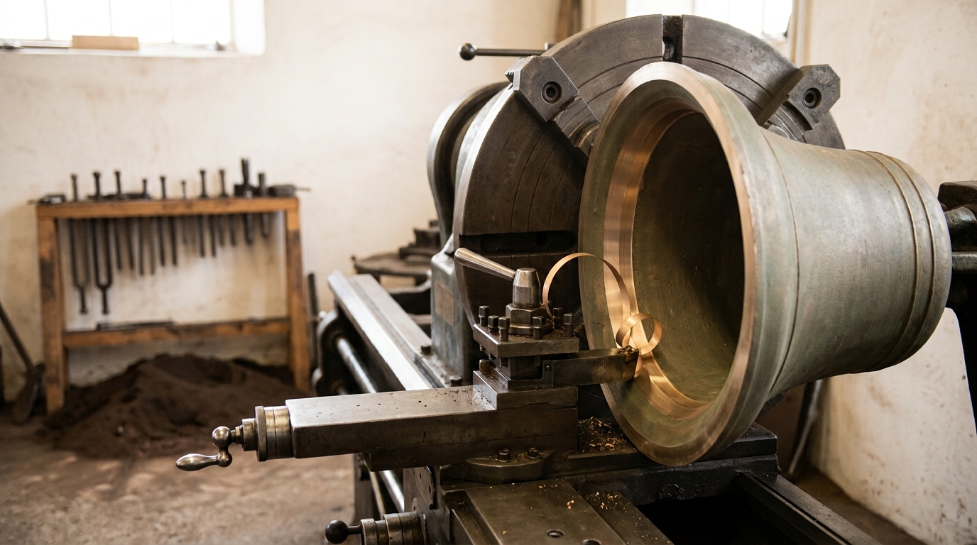
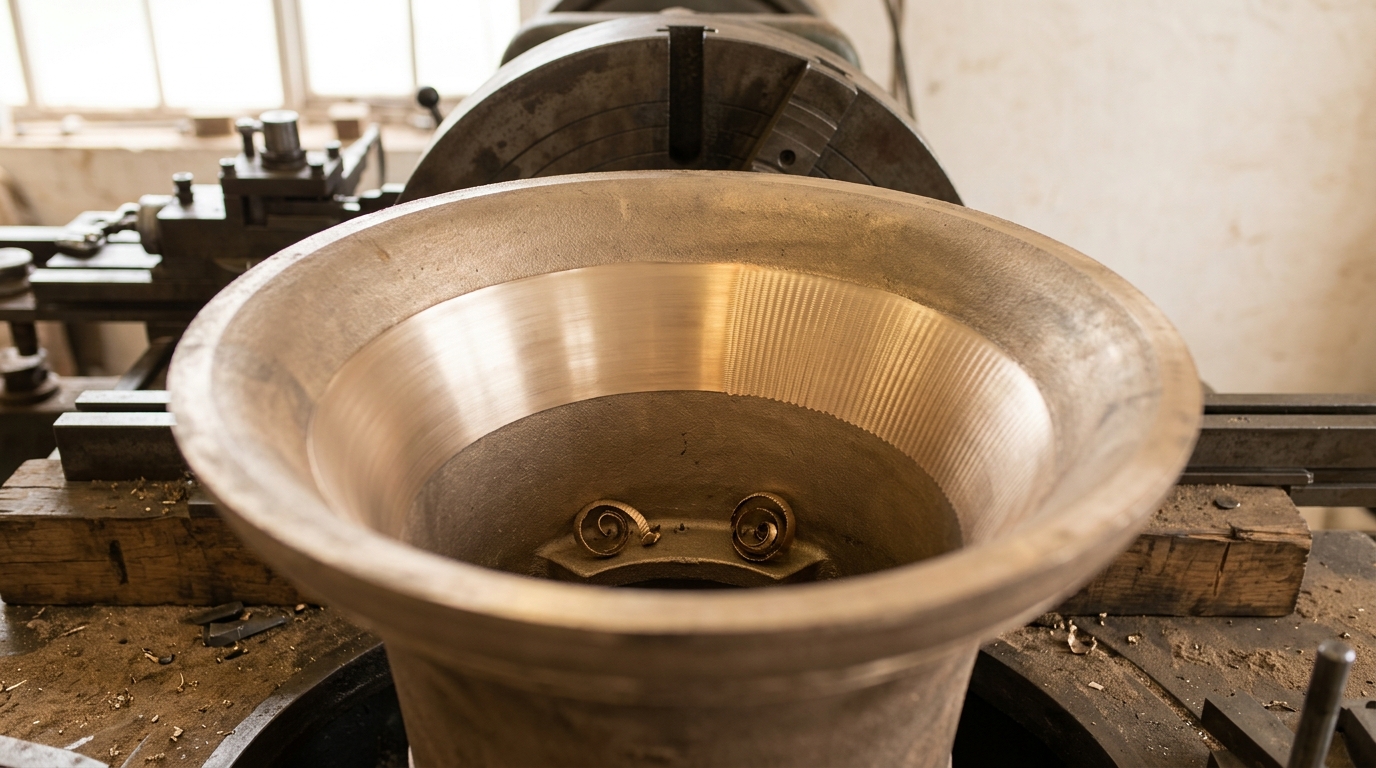
A bell foundry offers a better mental model than a chip fab. A cast bell is not in tune. Its partials — the hum, the prime, the tierce, the quint, the nominal — sit at ratios the founder cannot inspect from outside. The tuner mounts the bell mouth-up on a vertical lathe and shaves metal from the inner profile, sounding it against forks after each pass. The state of the bell is never observed directly; it is inferred from what the bell emits. Every correction spends bronze that cannot be replaced. Quantum error correction has the same structure, and the same economics.

Redundancy is forbidden, so something else has to be bought

The classical repetition code is the first thing anyone reaches for, and quantum mechanics forbids it. A unitary machine that maps an arbitrary unknown state alongside a blank register onto two copies,

cannot exist for all $|\psi\rangle$, because unitarity preserves inner products and the required map does not. Wootters and Zurek established the point in 1982, in a paper whose title remains the cleanest statement of it ^[1]. There is no backup copy, no parity check computed by reading the data, no majority vote over three inspected replicas.

Worse, quantum errors are continuous. A classical bit flips or does not. A qubit can be rotated by an arbitrary small angle, dephased partially, or entangled with a stray degree of freedom in the environment. The error space is not discrete, and enumerating it looks hopeless.

Shor’s 1995 code broke the deadlock by making two moves at once ^[2]. It spread one qubit of information across nine, so that no single physical qubit carries the state and no single physical qubit’s failure destroys it. And it showed that a code correcting bit flips and phase flips separately corrects any single-qubit error, because an arbitrary single-qubit operation decomposes over the Pauli basis and the syndrome measurement projects the continuous error onto one of its discrete components. Steane’s independent construction arrived the following year with a seven-qubit code and a general framework connecting quantum codes to classical linear codes ^[3]. Continuous errors become discrete not because nature is kind but because measurement discretises them.

Asking about the disagreement instead of the state

The technique that makes this work is the stabiliser formalism, given its general fault-tolerant treatment by Gottesman ^[4]. A code is defined not by listing its states but by naming a set of commuting Pauli operators $S_i$ — the stabiliser generators — whose joint $+1$ eigenspace is the code space:

An $[[n, k, d]]$ code encodes $k$ logical qubits into $n$ physical qubits with distance $d$. The stabiliser generators are measured repeatedly. Because each $S_i$ commutes with every other and with the logical operators, measuring them extracts no information about which encoded state is present. What it extracts is whether an error has anticommuted with a given check — a single classical bit per generator, per round. That bit string is the syndrome.

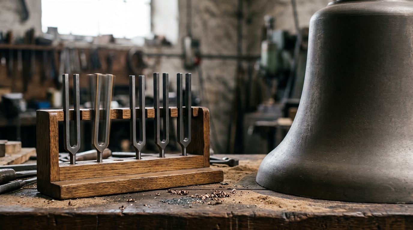
This is the conceptual core, and it is worth stating without hedging: the apparatus never learns the logical state, and therefore never collapses it. It learns only the pattern of disagreements between the object and a set of references. The tuner does not open the bell. A fork is struck beside it, and the beat between fork and bell reports the discrepancy. The bell’s actual sound is never transcribed.

Terhal’s review sets out the formalism and its memory-theoretic consequences in full, including the point that syndrome extraction is itself performed by faulty circuits and so must be repeated over many rounds before the syndrome record can be trusted ^[12]. A single round of checks measured with noisy gates and noisy readout produces a syndrome that is itself unreliable. Fault tolerance is not a property of a code; it is a property of a code together with a circuit that measures it and a procedure that interprets the result.

Physical and logical are different units of account

Distance $d$ is the weight of the smallest undetectable logical error. A distance-$d$ code corrects up to $\lfloor (d-1)/2 \rfloor$ errors. For the planar surface code in its standard rotated layout, the physical cost of one logical qubit is

counting data and measure qubits together. A distance-7 patch therefore occupies ninety-seven physical qubits, and that is a memory holding one logical qubit, doing nothing else. It performs no gate, produces no non-Clifford operation, and reserves no routing space.

The overhead is not a fixed multiplier. It is a function of how far below threshold the hardware sits and how long the algorithm must run, because the required logical error rate is set by the total number of logical operations. An algorithm with $10^{10}$ logical operations needs a logical error rate well below $10^{-10}$ per operation, and the distance required to reach that number depends on the physical error rate in a way examined in the next section. This is why “a thousand physical qubits per logical qubit” is a slogan rather than a specification: the true ratio depends jointly on $p$, on $d$, on the code, on the decoder, and on the depth of the computation being run.

What the threshold theorem does and does not promise

The threshold theorem is the reason the field exists. Stated informally: if the physical error rate per operation is below some constant $p_{\mathrm{th}}$ determined by the code, the noise model and the fault-tolerant circuit construction, then an arbitrarily long quantum computation can be performed with arbitrarily small error, at an overhead that grows only polylogarithmically in the size of the computation. Knill, Laflamme and Zurek established resilient computation under a constant error rate ^[5], and Aharonov and Ben-Or gave the constant-error-rate construction in a form that has become the standard citation ^[6].

What the theorem promises is asymptotic and conditional. What it does not promise is worth stating separately, because the gap between the two is where every real engineering programme lives.

It does not promise a specific threshold value. The number is not a constant of nature; it is a property of a triple — code, noise model, decoder. A depolarising-noise threshold quoted for one decoder does not transfer to circuit-level noise with a different one.

It does not promise that operating below threshold is sufficient. Below threshold, increasing $d$ suppresses logical error. The suppression is exponential in $d$ but the prefactor matters enormously in practice, and the useful regime is reached only when $p$ is well below $p_{\mathrm{th}}$, not marginally below it. Near threshold, the exponent is small and the overhead explodes.

It does not promise anything about correlated noise outside the assumed model. Leakage out of the computational subspace, crosstalk, drifting calibration and rare high-energy events all violate the independent-error assumptions in the standard proofs. The Google Quantum AI experiment that ran a distance-25 repetition code reported a logical error floor of $1.7 \times 10^{-6}$ per round set by a single high-energy event, falling to $1.6 \times 10^{-7}$ when that event was excluded ^[15]. That is a measurement of exactly the kind of correlated failure the theorems assume away.

The practical form of the promise is a scaling law. Below threshold, the logical error rate per round of a distance-$d$ code falls approximately as

so that each increase of the code distance by two multiplies the protection by a factor conventionally written

Below threshold means $\Lambda > 1$. Above threshold, adding qubits makes the logical qubit worse, because each additional physical qubit contributes more error than the larger code removes. This is the sense in which qubit count is not merely an incomplete figure of merit but can be an actively misleading one.

Why the surface code won on geography

Kitaev’s toric code introduced topological protection: logical information stored in global topological features of a two-dimensional lattice, with stabiliser checks acting only on neighbouring qubits ^[7]. Raussendorf and Harrington then gave a two-dimensional local fault-tolerant scheme and reported an error threshold of $0.75\%$ for each source in an error model including preparation, gate, storage and measurement errors ^[8]. The surface code descends from this line, and the review by Fowler, Mariantoni, Martinis and Cleland is the standard practical reference for its architecture, logical qubit construction and gate set ^[9].

The reason it dominates is not that its threshold is the highest imaginable. It is that its checks are geometrically local on a planar lattice with nearest-neighbour connectivity. Superconducting chips are planar. Lithography prefers planar. Wiring, control lines, and dilution refrigerator plumbing prefer planar. A code whose stabiliser generators require each qubit to interact with distant partners can have excellent parameters on paper and be unbuildable in the substrate that exists.

That constraint is a choice, not a law, and the alternatives are now concrete. Bravyi and colleagues at IBM presented a family of quantum low-density parity-check codes achieving an error threshold of $0.8\%$ for the standard circuit-based noise model, with a syndrome cycle requiring $n$ ancillary qubits and a depth-7 circuit of nearest-neighbour CNOT gates on a degree-6 connectivity graph made of two edge-disjoint planar subgraphs ^[19]. Their worked example preserves 12 logical qubits for nearly one million syndrome cycles using 288 physical qubits at a physical error rate of $0.1\%$, and they argue the surface code would need nearly 3000 physical qubits for the same suppression on 12 logical qubits. The comparison is an engineering estimate under a stated noise model, not a demonstrated device; but it shows that the overhead multiplier is a design variable rather than a constant.

Decoding is a classical computation with a deadline

The syndrome is a stream of classical bits produced every cycle. Something must convert that stream into a correction. This decoder is a classical algorithm running on classical hardware, and its performance requirements are severe in a way that is routinely omitted from popular accounts.

The decoder must be accurate, since a poor decoder lowers the effective threshold. It must also be fast enough, and this is the harder constraint. Syndrome rounds arrive continuously. If the decoder consumes each round more slowly than rounds are produced, its backlog grows without bound and the computation’s effective clock rate collapses. Because non-Clifford operations require a decoded result before the next gate can be chosen, the decoding latency enters the algorithm’s wall-clock runtime directly rather than being amortised away.

The Google Quantum AI below-threshold experiment reported a real-time decoder with an average latency of 63 microseconds at distance-5 sustained up to a million cycles, against a surface code cycle time of 1.1 microseconds ^[16]. Those two numbers, read together, are the whole of the real-time decoding problem in miniature. Earlier, a Honeywell Quantum Solutions team demonstrated repeated syndrome measurement on a ten-qubit trapped-ion QCCD processor using the $[[7,1,3]]$ colour code with a real-time decoder driving corrections applied either as Pauli-frame software updates or as physically applied gates ^[17]. The Pauli-frame technique — tracking the correction in classical software rather than applying it to the hardware — is one of the main ways the latency budget is bought back, and it works for Clifford operations precisely because Cliffords conjugate Paulis into Paulis.

Gidney and Ekerå’s resource estimate makes the timing assumptions explicit rather than burying them: a planar grid with nearest-neighbour connectivity, a characteristic physical gate error rate of $10^{-3}$, a surface code cycle time of 1 microsecond, and a reaction time of 10 microseconds ^[14]. That reaction time is the round trip from measurement to decoded decision to conditioned next gate. In their construction it is a first-class quantity in the runtime, not an implementation footnote.

The Clifford group is cheap; everything else is not

Surface codes protect Clifford operations relatively cheaply. Lattice surgery — merging and splitting code patches to implement multi-qubit measurements — gives a complete set of Clifford operations using only local operations on the planar lattice, and Litinski’s treatment reformulates large-scale surface code computation entirely in terms of qubits and measurements, avoiding braiding diagrams ^[11]. The problem is that Clifford circuits are efficiently simulable classically. A machine that performs only Clifford operations, however many logical qubits it holds and however long it holds them, computes nothing a laptop cannot.

Universality requires a non-Clifford gate, conventionally the $T$ gate. Non-Clifford gates cannot be implemented transversally in the surface code, and the standard workaround is magic state distillation, introduced by Bravyi and Kitaev ^[10]. Many noisy copies of a particular ancilla state are prepared, a Clifford circuit is applied, some are measured, and a smaller number of higher-fidelity copies survive. The output state is then consumed by gate teleportation to effect the $T$ gate.

The consequence for resource accounting is decisive. In published estimates for cryptographically relevant algorithms, the magic state factory dominates both the spatial footprint and the runtime. Gidney and Ekerå’s abstract circuit model — which, as they state, ignores overheads from distillation, routing and error correction — uses $3n + 0.002\, n \lg n$ logical qubits, $0.3 n^{3} + 0.0005\, n^{3} \lg n$ Toffoli gates and $500 n^{2} + n^{2} \lg n$ measurement depth to factor $n$-bit RSA integers ^[14]. It is the Toffoli count that sets the demand for distilled states, and it is the distillation of those states that turns a modest logical qubit count into the twenty million noisy physical qubits and eight hours of their title. The physical count is downstream of the non-Clifford count, not of the logical qubit count.

This is why a device’s qubit total tells you so little. Two machines with identical physical qubit counts can differ by orders of magnitude in useful capacity depending on their physical error rate, their cycle time, their decoder latency, and the fidelity of their distillation pipeline.

The honest state of below-threshold operation

Careful attribution matters here more than anywhere else in the field, because these results are frequently restated in forms their authors did not claim.

Google Quantum AI reported in 2023 the first experimental demonstration that logical performance improved with code size: a distance-5 surface code logical qubit modestly outperforming an ensemble of distance-3 logical qubits, with logical error per cycle of $2.914\% \pm 0.016\%$ against $3.028\% \pm 0.023\%$ ^[15]. The word “modestly” is theirs, and it is accurate. The margin was small; the significance was that the sign of the scaling had flipped.

The follow-up result reported a distance-7 surface code with $0.143\% \pm 0.003\%$ error per cycle of error correction, an error suppression factor of $\Lambda = 2.14 \pm 0.02$ when increasing the code distance by two, and a logical qubit lifetime exceeding the best physical qubit’s lifetime by a factor of $2.4 \pm 0.3$ ^[16]. That is a memory experiment at a single logical qubit. It is a genuine threshold crossing and it is not a computation.

On a different hardware platform, a Harvard, MIT and QuEra collaboration reported a processor based on encoded logical qubits operating with up to 280 physical qubits in reconfigurable neutral atom arrays, demonstrating improvement of a two-qubit logic gate by scaling surface code distance from $d=3$ to $d=7$, operation of 40 colour code qubits, and sampling circuits with up to 48 logical qubits entangled with 228 logical two-qubit gates and 48 logical CCZ gates using three-dimensional $[[8,3,2]]$ code blocks ^[18]. The $[[8,3,2]]$ code has distance 2: it detects errors without correcting them. Reporting 48 logical qubits is correct; reading it as 48 fault-tolerant qubits at algorithmic distance is not.

The pattern across all three is the same. Memory has crossed below threshold on at least one platform at modest distance. Logical operations have been demonstrated at small scale and low distance. Sustained, decoded, magic-state-supplied logical computation at the distances an algorithm needs has not been demonstrated by anyone, and none of these papers claims it.

Vendor roadmaps projecting particular logical qubit counts by particular years are announcements of intent. They are not experimental results, they are not theorems, and they should not be cited as either.

The unit that should be quoted

If physical qubit count is the wrong figure, what replaces it? The honest answer is a product with four factors: how many logical qubits a machine can hold, at what distance, for how long, while supplying non-Clifford states at what rate. Compressed to a single quantity, it is logical qubit-seconds after overhead — the integral of protected, decoded, usable logical registers over wall-clock time, with the magic state supply treated as part of the machine rather than as an accessory to it.

Under that unit, several familiar claims change character. A processor with a thousand physical qubits at a physical error rate above threshold has a capacity of zero, because increasing its code distance would make matters worse. A processor with fewer qubits but a physical error rate an order of magnitude below threshold has real capacity, because distance buys suppression. A processor with excellent qubits and a decoder that cannot keep pace with the syndrome stream has capacity limited by classical electronics rather than by physics.

The bell tuner’s discipline is exactly this. The bell cannot be inspected; it can only be sounded. Each pass of the tool is inferred from the disagreement between the emitted partials and the forks, and each pass spends bronze irreversibly. A tuner who reported progress by the mass of the casting would be measuring the wrong thing entirely. What matters is how close the partials now sit to true, and how much wall thickness remains to keep correcting with.

Error correction is not the tax levied on quantum computing before the interesting part begins. Between the no-cloning theorem and the resource estimates, it is the mechanism by which anything at all becomes computable on hardware that decoheres. It is the whole problem, and the number that measures progress against it is not on the front of the press release.