Edge AI Electronics and Sensor Systems: A First-Principles Introduction

Two ends of one wire

A large language model answering a question and a hearing aid cancelling wind noise are both, in the loosest sense, “AI.” Treating them as points on the same curve is the single most common mistake in popular writing about edge AI. They are closer to opposite ends of a wire.

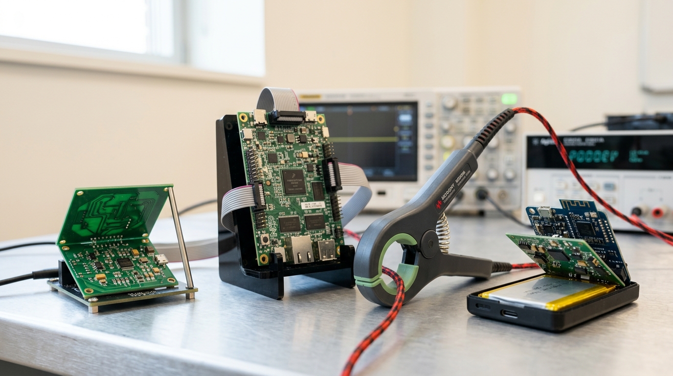
At one end sits a data center: effectively unbounded electrical supply, active liquid or forced-air cooling, elastic compute that can be added by the rack, and a network path back to the user that costs tens to low hundreds of milliseconds. At the other end sits a battery-powered, coin-sized, often single-chip system that must sense the world, decide something about it, and act — on a power budget measured in microwatts to a few hundred milliwatts, with a memory budget measured in kilobytes to a few megabytes, and with no guarantee that a network is present at all. A vibration sensor bolted to a pump bearing, a camera trap in a forest with no cellular signal, an implanted or wearable biosensor, a smoke detector that must not go silent when a subscription lapses — all of these need to make a decision locally, because sending the raw signal elsewhere is not merely inconvenient but frequently impossible, too slow, too power-hungry, or too invasive of the thing being sensed.

This is not a smaller version of the cloud problem. It is a different problem that happens to use some of the same mathematics. Moving inference from a data center to the point of sensing does not just shrink the model; it inverts which resources are scarce. In the cloud, the scarce resource is usually money, expressed as compute-hours. At the edge, the scarce resources are physical and unforgiving: the energy stored in a cell that may need to last a year without replacement, the milliseconds available before a control decision is late, and the fact that raw sensor data — a voice, a face, a heartbeat — is the kind of information a system should arguably never transmit in the first place.

This article is the first in a series on edge AI electronics and sensor systems. Its job is not to cover any one of those constraints in depth — later pieces in this series do that — but to lay out the physical anatomy every one of those later articles assumes, and to define, carefully and from first principles, the handful of terms that vocabulary keeps returning to: TOPS per watt, quantization, always-on sensing, analog front ends, and event-driven readout.

The anatomy of an edge AI system

Strip away the specific application and almost every edge AI system reduces to the same three-stage chain.

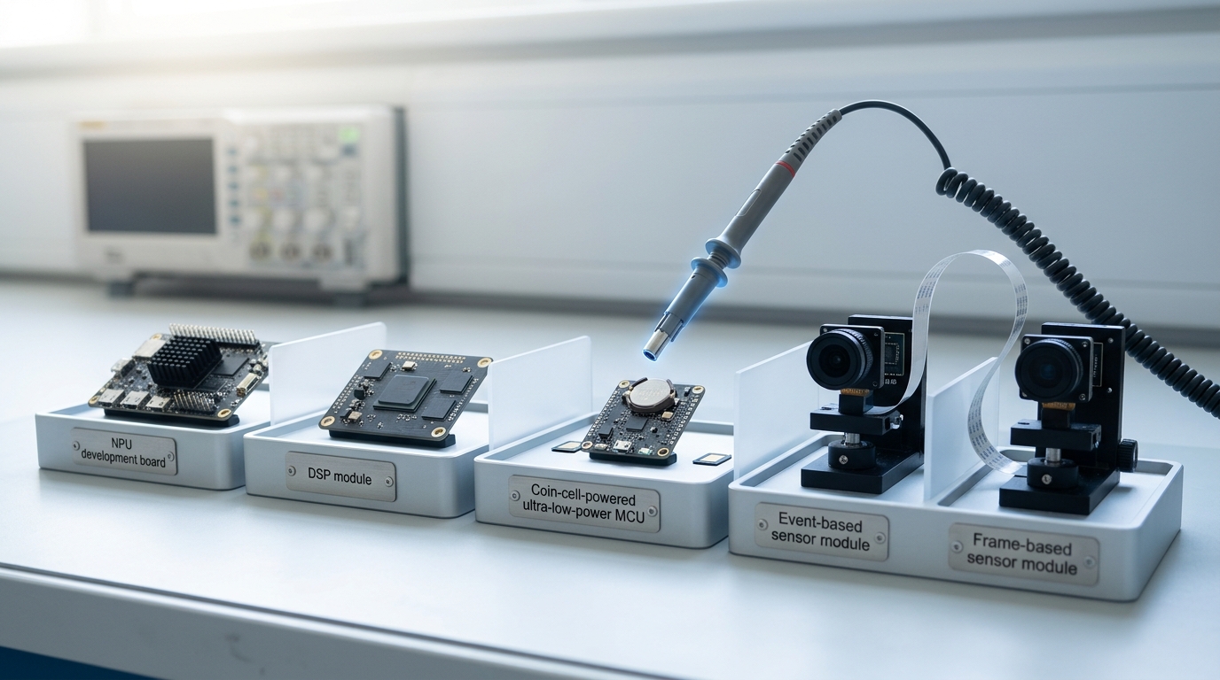
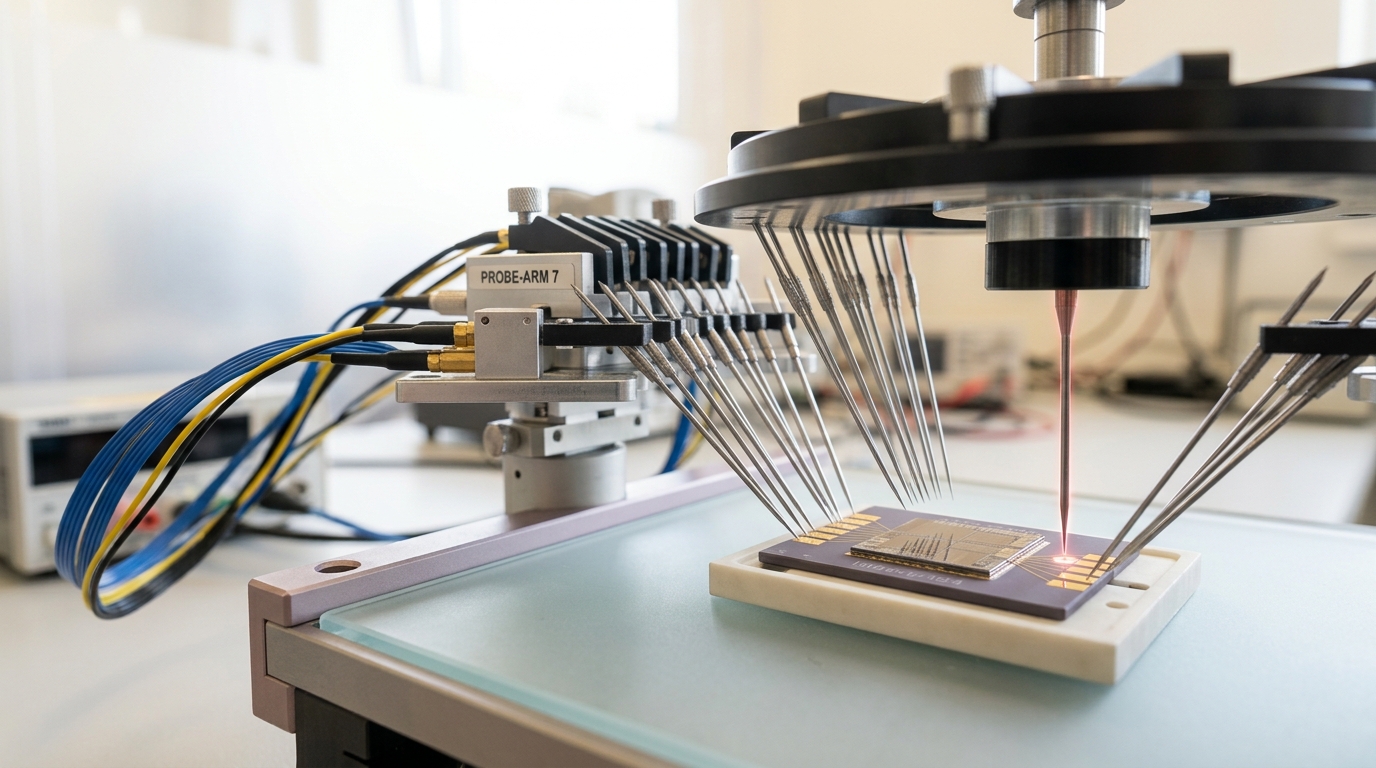
First, a sensor: a physical transducer that converts some quantity in the world — light intensity, sound pressure, acceleration, magnetic field, gas concentration, temperature — into an electrical signal, almost always a very small analog voltage or current. Second, an analog front end (AFE): a chain of amplification, filtering, and analog-to-digital conversion that turns that small, noisy, continuous signal into a clean, discrete stream of digital samples an embedded computer can work with. Third, an embedded processor, frequently paired with a dedicated neural processing unit (NPU) or other fixed-function accelerator, that runs a trained model against those samples and produces a decision, a classification, or a control signal, all within a power and memory envelope fixed at design time rather than provisioned on demand.

None of these three stages is optional, and the boundary between them is where most of the engineering difficulty in this whole field concentrates. A processor is only as good as the samples it receives; an analog front end is only as good as the sensor signal it is given to condition; and a sensor’s raw output is close to meaningless until the other two stages have acted on it. Vivienne Sze and colleagues, in the tutorial and survey that remains one of the most cited references on efficient neural network hardware, frame the processor stage specifically around this constraint: DNN hardware efficiency is not a property of an algorithm in the abstract, it is a joint property of the algorithm, the numerical representation it runs in, and the architecture that moves data to and from arithmetic units ^[1]. The same logic runs backward through the whole chain. Design decisions made in the sensor and the front end determine what the processor is even asked to do.

From a physical quantity to a number: the sensor and its analog front end

A microelectromechanical (MEMS) microphone’s diaphragm moves by nanometers in response to sound pressure. A photodiode produces a photocurrent measured in picoamps to nanoamps under typical ambient light. A capacitive accelerometer’s proof mass shifts a capacitance by femtofarads under normal motion. None of these raw signals is directly usable. They are small relative to circuit noise, they are continuous in time and amplitude, and they typically ride on top of an offset or bias that itself drifts with temperature and supply voltage.

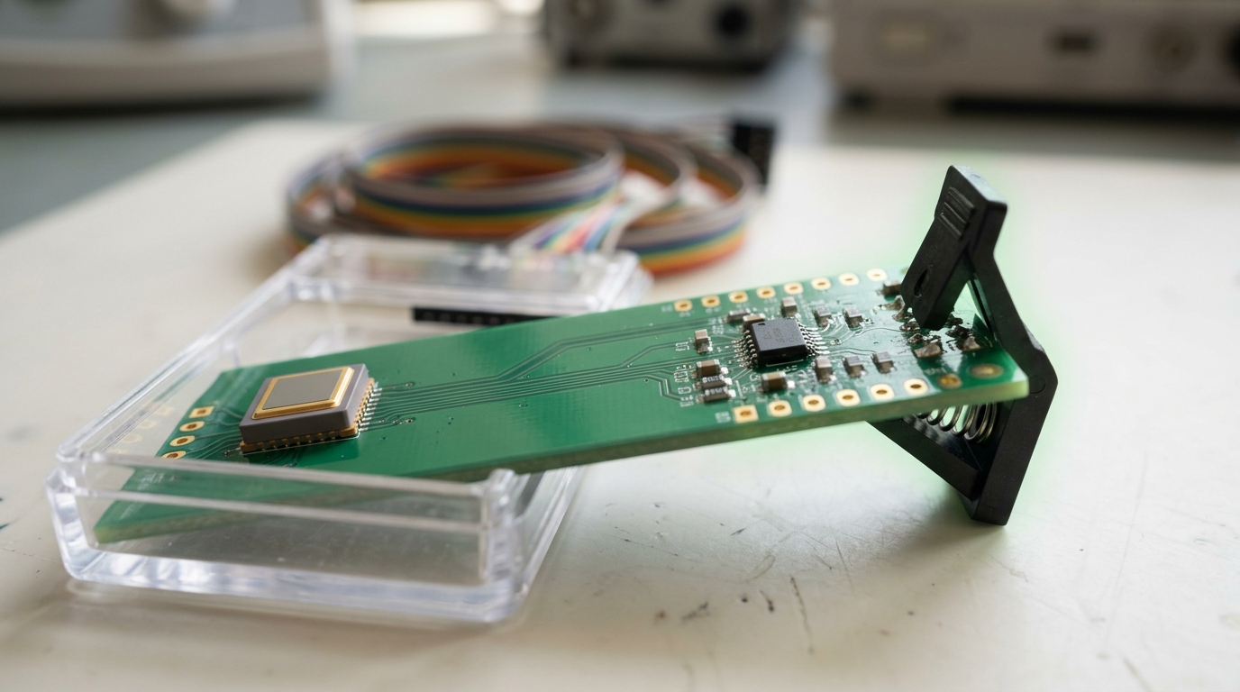
The analog front end exists to close that gap. A typical AFE chain amplifies the signal to a usable voltage range, filters out frequencies the application does not care about (both to remove noise and to prevent aliasing before sampling), and then digitizes it with an analog-to-digital converter (ADC) whose resolution and sample rate are chosen to match the sensor’s actual information content rather than some generic default. Kwantae Kim and Shih-Chii Liu’s review of continuous-time analog filter circuits for audio edge devices makes a point that generalizes well beyond audio: pushing filtering and feature extraction earlier into the analog domain, before digitization, can substantially cut the power spent moving and processing samples that a digital pipeline would otherwise have to touch one by one ^[6]. This is a design trade specific to the edge. In a data center, discarding information early to save power is rarely worth the engineering cost; at the edge, it is frequently the difference between a device that lasts a year on a coin cell and one that does not last a week.

This boundary between the physical and digital worlds is also where standardization becomes relevant, because a sensor and its front end are not always designed by the same team, or even the same company, as the processor consuming their output. The IEEE 1451 family of standards addresses exactly this seam: a common, network-independent way for a “smart transducer” to describe itself — its type, its calibration, its native units — to whatever system reads it, via a small attached data structure called a Transducer Electronic Data Sheet ^[8]. Whether or not a given product actually implements IEEE 1451, the problem it solves is universal: a processor cannot make good use of a sample unless it knows, unambiguously, what physical quantity that sample represents and under what conditions it was taken.

The processor, and what “TOPS per watt” actually measures

Once digitized samples exist, the third stage — the embedded processor — runs a trained model over them. Two numbers dominate how that stage is described, and both are frequently misused.

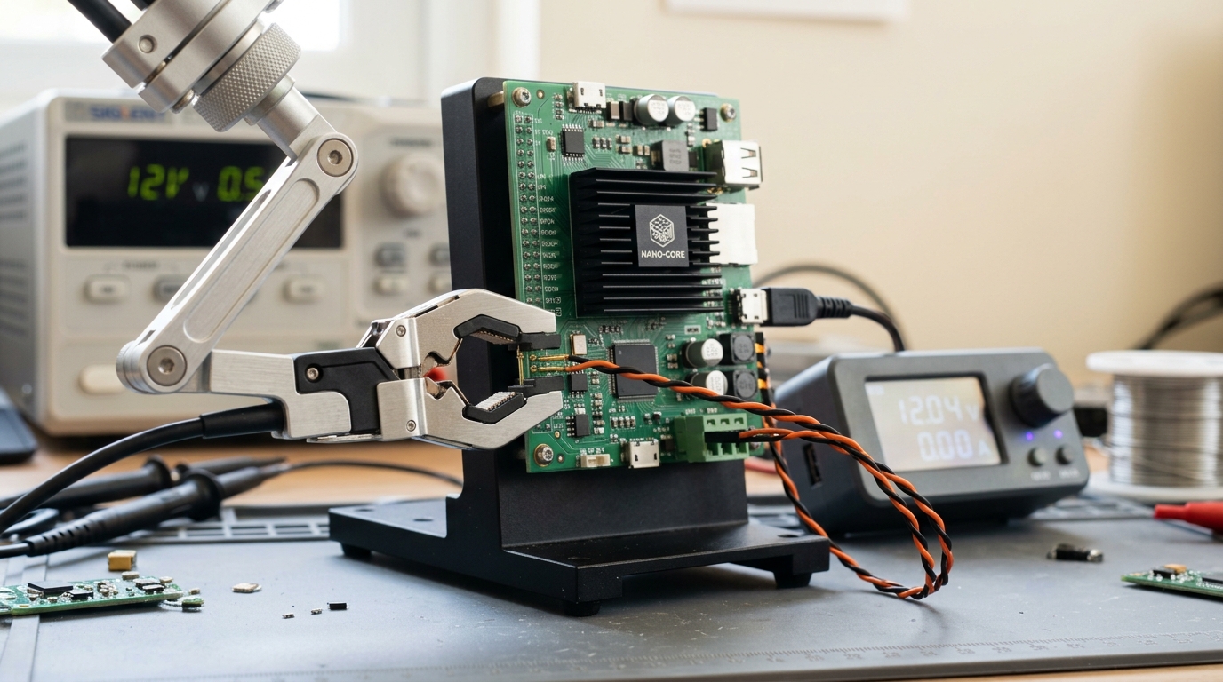
TOPS, tera-operations per second, measures raw throughput: how many multiply-accumulate operations a chip can, in principle, perform in a second. It says nothing about power, and by itself it is close to useless for comparing edge hardware, because a processor is free to spend arbitrarily large power to hit a large TOPS number. The metric that actually matters for a battery-powered or thermally constrained device is efficiency — operations delivered per unit of energy, conventionally reported as TOPS per watt:

Because a watt is a joule per second, $\eta$↗ measured this way is numerically the same quantity as operations delivered per joule. That equivalence matters because it converts a throughput specification into an energy budget for a single inference:

where $N_{\text{ops}}$↗ is the number of operations one inference requires. This is the arithmetic that determines whether a given model can run a given number of times on a given battery before it needs replacing or recharging, and it is why a headline TOPS figure on a datasheet, quoted without the power draw it was measured at, tells a reader almost nothing about whether a part is suitable for a battery-powered product.

Two things move $\eta$↗ in practice, and both are visible in the published record rather than being vendor marketing claims. The first is architecture: Yu-Hsin Chen, Tushar Krishna, Joel Emer, and Vivienne Sze’s Eyeriss accelerator demonstrated that a “row-stationary” dataflow — one that keeps partial sums and weights resident in local memory rather than repeatedly re-fetching them from off-chip DRAM — could deliver roughly an order of magnitude better energy efficiency than a comparable mobile GPU on the same convolutional workload, purely from reducing data movement, without a smaller manufacturing process ^[5]. Data movement, not arithmetic, dominates the energy cost of running a neural network on real hardware, and that fact is the organizing idea behind essentially all edge accelerator design.

The second lever is numerical precision. Benoit Jacob and colleagues’ integer-quantization scheme showed that running inference with 8-bit integer arithmetic instead of 32-bit floating point — with a matched training procedure to control the resulting accuracy loss — cuts memory footprint roughly fourfold and substantially improves the latency-versus-accuracy trade-off on commodity ARM processors ^[3]. Quantization, in this sense, is not a compression trick applied after the fact; it is a design decision about how few bits are spent representing each weight and activation, made because every bit read from memory and pushed through an arithmetic unit has an energy cost, and the edge is the one setting in this entire field where that cost is felt directly, on a battery, rather than absorbed into a data center’s electricity bill. At the most constrained end of this spectrum, Ji Lin and colleagues’ MCUNet system co-designs both the model and the inference engine specifically for microcontrollers with only a few hundred kilobytes of memory — two to three orders of magnitude less than a mobile phone — demonstrating that useful vision models can run within that envelope when the architecture, quantization, and memory scheduling are all treated as one joint problem rather than three separate ones ^[10].

Power budgets and always-on sensing

Many of the most useful edge applications are not triggered by a button press; they must watch continuously for an event that might never come — a wake word, an intrusion, a fall, a machine fault — and they must do so for months or years on a fixed energy store. This is the always-on sensing problem, and it is fundamentally a duty-cycling problem: the system spends most of its life in a low-power idle or listening state and only occasionally, briefly, enters a higher-power active state to run full inference.

The average power such a system draws follows directly from how much time it spends in each state:

where $D$↗ is the fraction of time spent active. Because $P_{\text{active}}$↗ is typically one to three orders of magnitude larger than $P_{\text{idle}}$↗ for a real accelerator, battery life is dominated almost entirely by $D$↗ and by $P_{\text{idle}}$↗ — not by how efficient the processor is once it wakes up. This is precisely why an always-on product design effort spends so much of its attention on cheap, low-power triggering stages (a simple always-listening front end that only wakes the expensive processor when something resembling the target event occurs) rather than on the accelerator’s peak TOPS figure, which only matters for the small fraction of time $D$↗ actually represents.

This is also why standardized, energy-aware benchmarking matters for this class of device specifically. The MLPerf Tiny benchmark suite, assembled by a working group spanning more than fifty organizations across academia and industry, measures latency, energy, and accuracy together rather than accuracy alone, precisely because a model that is marginally more accurate but draws meaningfully more energy per inference can be the worse product choice for a duty-cycled, battery-powered application even though it would win on a conventional accuracy leaderboard ^[4]. Treating energy as a first-class benchmark axis, not an afterthought, is one of the clearest markers separating edge machine learning practice from cloud machine learning practice.

Event-driven sensing: a different anatomy for the same job

Everything described so far assumes a sensor that samples on a fixed clock — a microphone or accelerometer producing a new value every so many microseconds regardless of whether anything changed. There is a second family of sensors that inverts this assumption entirely: event-driven sensors, of which the best-studied example is the event camera or dynamic vision sensor.

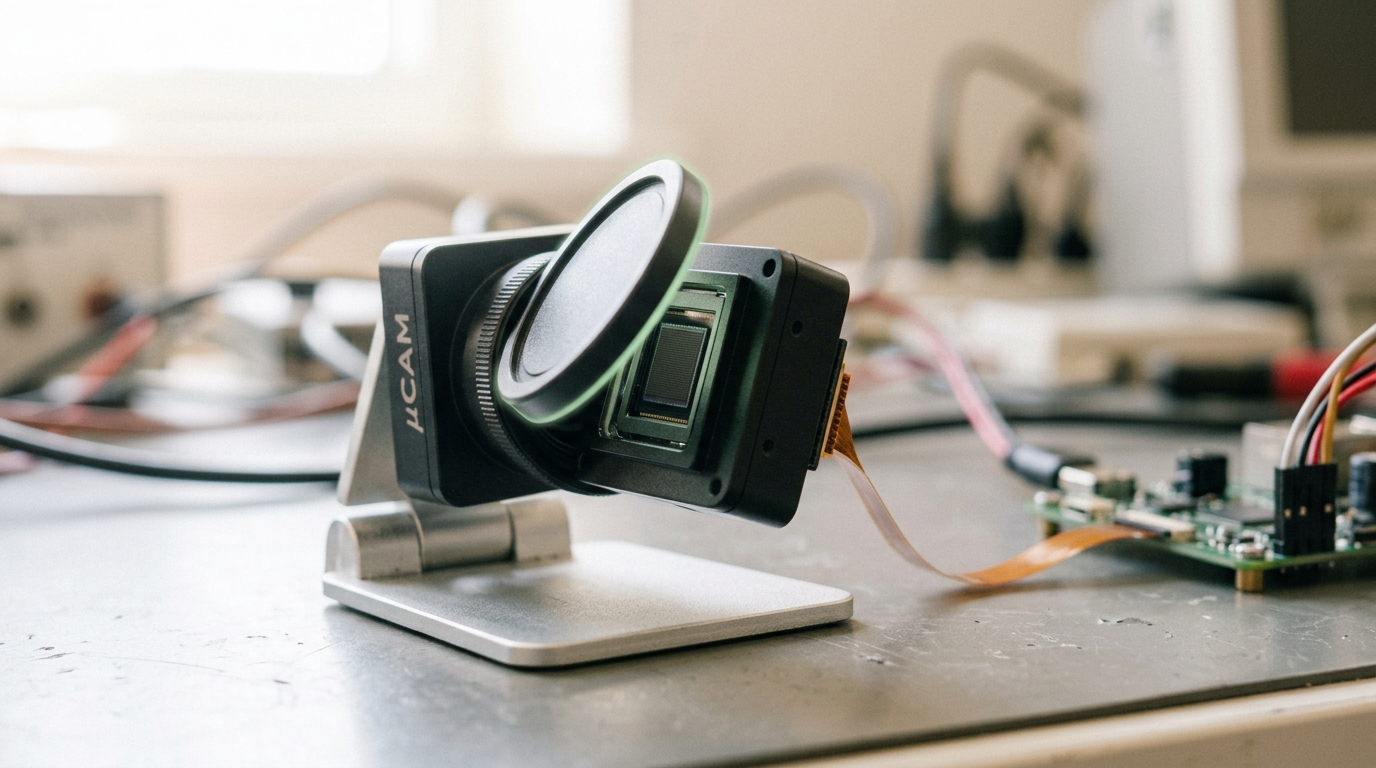
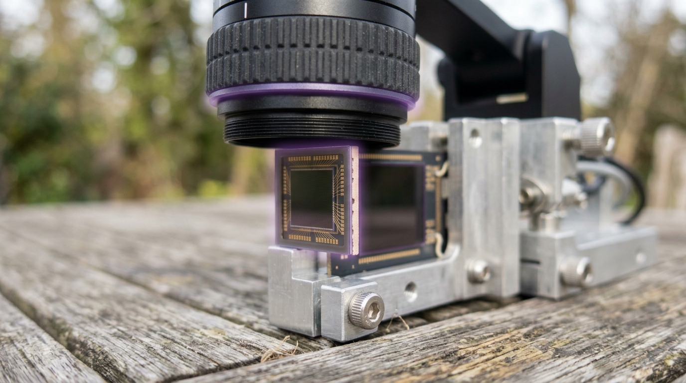
An event camera does not capture frames. Each pixel operates independently and asynchronously, reporting a small packet of information — its address, a timestamp, and the sign of the change — the instant its local brightness changes by more than a threshold, and staying silent otherwise. Guillermo Gallego and colleagues’ survey of the field, spanning contributions from more than a decade of hardware and algorithm development, catalogs the resulting properties: microsecond-scale temporal resolution, dynamic range exceeding 120 decibels versus roughly 60 decibels for a conventional frame sensor, and — the property most relevant to this article — a data rate and power draw that scale with how much is actually changing in the scene rather than with a fixed frame rate applied uniformly regardless of content ^[2]. A static scene produces close to no output at all; a sensor watching an empty hallway spends almost nothing, while one watching a busy intersection reports proportionally more.

That property reshapes where the power and latency budgets in the rest of the chain get spent. A conventional camera pipeline pays a roughly constant cost to acquire and process every frame whether or not anything of interest occurred in it. An event-driven pipeline concentrates that cost onto the moments something is actually happening, which is a good match for exactly the always-on, mostly-quiescent workloads described in the previous section. The trade is not free — event data requires processing algorithms genuinely different from frame-based computer vision, and much of the survey’s length is devoted to that adjustment — but the underlying idea, sampling proportional to information content rather than to a fixed clock, recurs often enough across sensor modalities in this series that it is worth introducing here as a general principle rather than a camera-specific curiosity.

Latency and control: the round trip you cannot afford

A second constraint separates edge systems from cloud ones even when power is not the binding limit: some decisions have a deadline measured in microseconds to low milliseconds, driven by physics rather than by user patience. A closed feedback control loop — stabilizing a drone, cancelling acoustic feedback in a hearing aid, tripping a machine safety interlock — must sense, decide, and act within a window set by how fast the underlying physical process moves. Round-tripping that decision to a remote server adds network latency that is not just larger than the available window, it is also variable, and a control loop that is fast on average but occasionally late is often worse than one that is uniformly slower, because the failure mode of a missed control deadline is not a delayed answer but an unstable system.

This is one of the two structural reasons — privacy, discussed next, is the other — that “just send it to the cloud and send the answer back” is not a scaled-down inconvenience for these applications but a category error. The inference has to happen where the actuation happens, on hardware whose worst-case timing, not just its average timing, is known at design time. It is also why interoperability standards for the sensing layer, like IEEE 1451’s data model for describing a transducer’s calibration and units in a form a control system can consume deterministically, matter more at the edge than they might appear to from a purely software vantage point: a control loop cannot afford to discover at runtime what a sensor’s units are or whether its calibration has expired ^[8].

Privacy is decided by where the wire goes

On-device inference is frequently marketed as a privacy feature, and the underlying claim is often true, but it is worth stating carefully rather than taking on faith, because “processes on-device” is a vendor assertion until a specific system’s data flow has been examined. The relevant fact is architectural, not promotional: if raw audio, video, or biometric data is converted into a decision locally and only that decision — not the raw signal — ever leaves the device, then the raw signal simply does not exist anywhere it could later be intercepted, subpoenaed, or breached. That is a stronger property than a policy promising not to retain data that was, in fact, transmitted.

Reza Shokri and Vitaly Shmatikov’s early work on privacy-preserving deep learning is a useful reference point here because it draws exactly this architectural distinction formally: a system in which participants share only model parameter updates, rather than raw training data, changes what an attacker positioned on the network can ever observe, even though it does not eliminate every inference risk on its own ^[7]. The edge case of that idea is the simplest possible privacy architecture — a device that never transmits the sensor signal at all because the entire model runs locally — and it is why “runs on-device” is a substantively different and generally stronger claim than “encrypts data in transit,” even though both are frequently marketed under the same “privacy” heading.

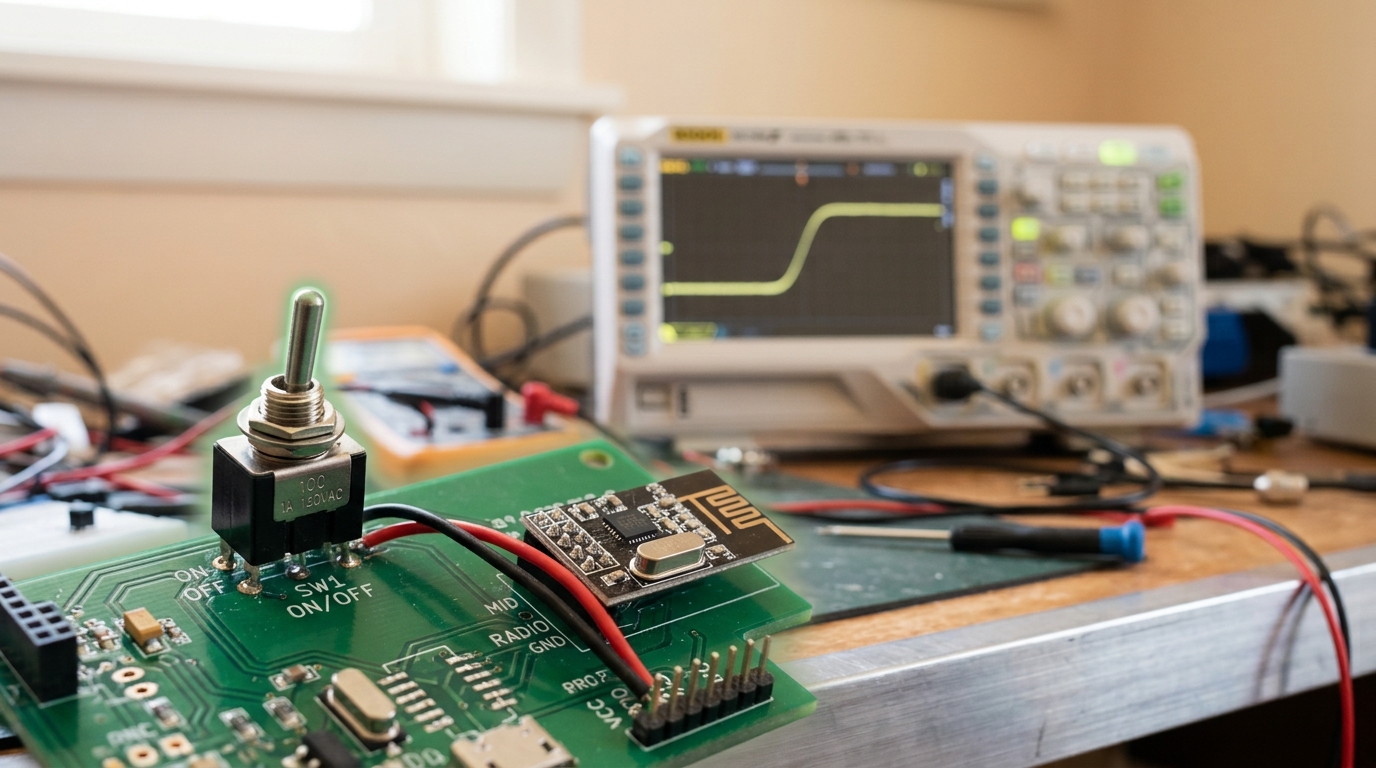
None of this is automatic, and it does not remove the need for conventional device security. NIST’s IoT Device Cybersecurity Capability Core Baseline lists data protection, along with device identification, configuration management, and secure logical access, as one of a small set of technical capabilities a securable IoT device needs regardless of where its inference happens ^[9]. On-device inference narrows what could leak; it does not, by itself, secure the device that holds it, and a system whose model can be extracted or whose local storage is unencrypted has traded one exposure for another rather than removed it. The strongest version of the architectural claim — the one this series will return to — is a hardware cutoff placed ahead of the radio: a physical switch that a line of firmware, however compromised, cannot silently re-enable.

Field reliability: what the demonstration bench skips

Every number in this article so far describes a system on a bench, freshly calibrated, at a stable ambient temperature, with a fresh battery. Deployed edge sensors do not stay in that state, and the gap between bench performance and field performance is one of the least glamorous but most consequential topics in this whole domain.

Sensors drift. A gas sensor’s baseline shifts with humidity and age; an accelerometer’s zero-offset moves with temperature cycling; a microphone’s sensitivity changes as dust or moisture accumulates on its port. Tiago Veiga and colleagues’ study of low-cost air-quality sensor networks measured this directly: even sensors calibrated correctly at deployment accumulated a long-term, unidirectional drift over months in the field, and the paper’s blind-calibration approach — inferring and correcting that drift from the correlation structure across many co-located sensors, without ever revisiting each unit physically — reported reconstructing the true signal well enough to keep mean-square error under 10% on real deployment data where naive uncorrected readings had drifted far outside that bound ^[11]. A model trained and validated on clean, freshly calibrated sensor data can degrade in the field for reasons that have nothing to do with the model at all — the input changed character even though the world being measured did not.

Batteries age and their usable capacity falls with cycle count and cold temperature; connectors corrode; enclosures that are perfectly sealed on day one accumulate seal fatigue over years outdoors. None of this shows up in a lab demonstration, which is exactly why a first-principles account of edge AI electronics has to name it explicitly rather than let the reader assume that a system validated once, in a controlled setting, stays validated for its full deployed lifetime.

A working vocabulary for the rest of this series

Collected in one place, the terms this article has built up: TOPS/W is operations delivered per unit of energy, the efficiency metric that actually governs battery life, distinct from and often more important than raw TOPS. Quantization is the choice of how few bits represent each weight and activation, traded deliberately against accuracy because every bit read and computed costs energy. Duty cycling is the practice of spending most of a device’s life in a low-power state and only briefly entering a high-power active state, and it is the dominant lever on average power for always-on sensing applications. An analog front end (AFE) is the amplification, filtering, and conversion chain that turns a raw, small, noisy sensor signal into digital samples a processor can use. Event-driven sensing samples in proportion to how much is actually changing in the world rather than on a fixed clock. And privacy at the edge is best understood architecturally — by tracing which signals a device transmits and which it decides never to — rather than by the presence of a privacy statement.

Signals to watch, and what would falsify them

Three modest, falsifiable expectations for how this field moves over the next few years, stated with the assumptions and disconfirming evidence they depend on.

One. Published efficiency comparisons across edge processors will increasingly report TOPS/W at a stated, specific workload and precision rather than as a single peak figure, because peak-figure comparisons across differently quantized workloads have already become indefensible following results like Jacob and colleagues’ ^[3] and the workload-matched methodology MLPerf Tiny was built to enforce ^[4]. Horizon: three years from publication. Disconfirmed if major processor datasheets in that window still report a single unqualified TOPS/W figure with no stated precision or benchmark.

Two. Event-driven and duty-cycled always-on sensing will keep expanding into modalities beyond vision and audio — gas sensing, vibration, biosignals — because the underlying argument (spend energy in proportion to information content rather than on a fixed clock) does not depend on the sensing modality. Horizon: five years. Assumption: the manufacturing cost premium for event-driven front ends over conventional clocked sampling continues to fall. Disconfirmed if event-driven architectures remain confined to vision after five years despite falling component costs.

Three. The gap between bench-reported accuracy and field-measured accuracy for deployed sensor-driven models will remain a persistent, separately reported number in serious engineering literature, rather than closing — because drift, as Veiga and colleagues measured it, is a property of the physical sensor and its environment, not of the model ^[11]. Disconfirmed if a majority of new deployment studies in this space report field accuracy matching bench accuracy within measurement noise, without an explicit recalibration step.

None of these predictions requires a hardware breakthrough. They follow from the anatomy already laid out here: a signal chain of sensor, analog front end, and processor, each governed by a physical budget — energy, time, or information — that a data-center system simply does not have to answer to in the same way.