A model that runs correctly on a bench, tethered to a lab supply, in a climate-controlled room, has answered none of the questions that decide whether an edge AI sensor system survives being deployed. The deployment questions are different in kind: how many years can this run on the battery or panel it shipped with; how much has the sensor drifted by the time anyone next opens the enclosure; and what, specifically, is allowed to leave the device at all. This guide works through those three questions in the order a field engineer actually meets them — power, drift, and privacy — and treats every number as either a verified standard, a measured study, or an explicitly labeled vendor claim. Where a claim is analysis rather than fact, or a prediction rather than either, that is said plainly, because the failure mode in this domain is rarely a wrong number; it is an unlabeled one.
The power budget is not a spec-sheet subtraction
The naive power budget for an always-on edge AI sensor node is a subtraction: battery capacity in milliamp-hours, divided by average current draw, gives a service life in hours. In practice this number is wrong by a large factor in almost every field deployment, for reasons that are individually well understood and collectively under-modeled.
The first reason is that “always-on” inference is not a single power state. A wake-word or anomaly-detection pipeline spends the overwhelming majority of its time in a cheap, low-accuracy monitoring stage — an analog voice-activity detector or a coarse motion threshold — that only escalates to a full neural network inference when something looks interesting. Hello Edge, the foundational study on keyword spotting for microcontrollers, established the accuracy/footprint trade curve that this staging strategy is built on: small convolutional and recurrent models can hit usable wake-word accuracy within the memory and compute envelope of a Cortex-M class microcontroller, but only if the network itself runs rarely [8]. A subsequent line of work pushed the always-on stage itself down into sub-milliwatt analog front-ends, reporting a design that performs binary feature extraction and a binary neural network classifier in the sub-milliwatt range specifically so that the power-hungry digital core can stay asleep almost all the time [10]. The industry-standard way to compare these design points is MLPerf Tiny, which defines TinyML explicitly as inference under roughly one milliwatt of active power on embedded hardware and measures accuracy, latency and energy together rather than accuracy alone, precisely because a model that is 2 percent more accurate at ten times the energy cost is not a win in a battery-budget sense [3]. The practical consequence for a field engineer is that the number worth optimizing is not “inference cost” as a single figure but the duty cycle: what fraction of total device time is spent in each power state, and how expensive is the escalation trigger that promotes work from one state to the next.
The second reason the naive subtraction is wrong is that battery capacity itself is not constant. Lithium-based chemistries lose usable capacity with temperature, discharge rate and calendar age, and a field node mounted on an outdoor pole experiences all three simultaneously in ways a lab test rarely reproduces. This is a case where the honest move is to say what is not established here: manufacturer capacity-fade curves are vendor claims, not independently verified measurements, and this article does not have a peer-reviewed field study of pole-mounted edge AI battery fade to cite specifically — the closest verified evidence is the aging and reliability literature on the electronics themselves, covered below. Where a deployment’s power budget rests on a vendor’s fade curve, that dependency should be stated as a vendor assertion in the design documentation, not folded silently into a service-life number presented as fact.
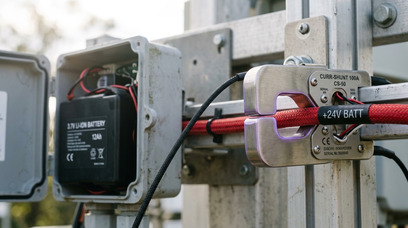
The third reason is that measurement itself has a cost and a failure mode. A current-sense shunt clamped around the supply rail is the standard way to verify what a design is actually drawing, as opposed to what its datasheet implies, and the discipline of doing this at multiple points in the duty cycle — sleep, wake-trigger evaluation, full inference, radio transmission — is what turns a power budget from arithmetic into an engineering artifact someone can defend. A budget built only from datasheet typical-current figures, without a bench measurement at each state, is analysis built on unverified vendor numbers stacked several layers deep; a single shunt measurement campaign, even a short one, converts most of that stack into fact.
Here
Drift is not a defect; it is the normal operating condition
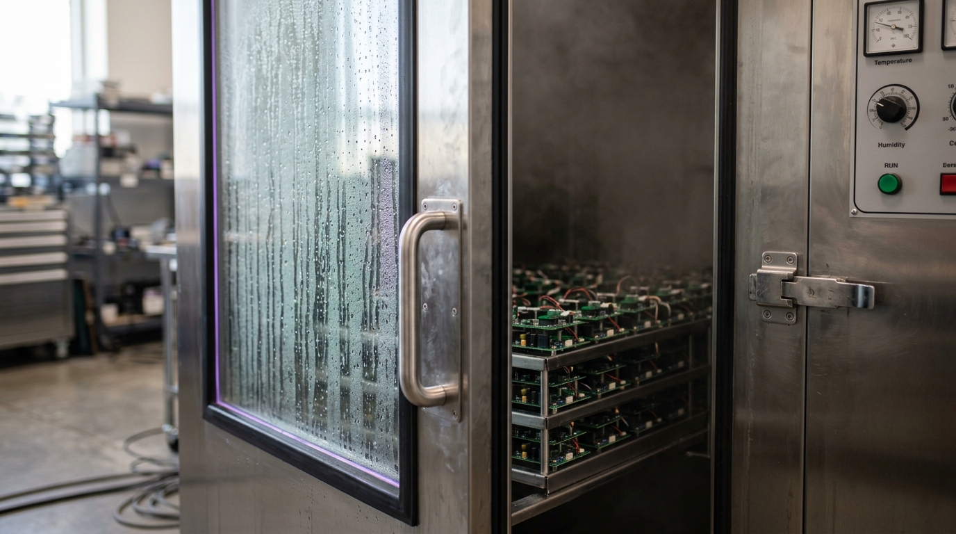
A sensor node that ships calibrated and correct will not stay that way. This is not a failure mode to be engineered around in the sense of eliminating it; it is a normal operating condition to be engineered around in the sense of bounding and, where possible, correcting it in the field.
MEMS inertial sensors are the best-measured case. A study of natural aging in
biaxial MEMS accelerometers tracked commercial devices over roughly ten and
four years respectively and found offset and scale-factor drift reaching
about 2.6 percent and 1 percent of full scale in the two devices measured,
attributing the drift to slow mechanical and material aging in the sensing
structure itself rather than to any single discrete failure
[5]. A separate accelerated-aging study
measured the mismatch in sensitive capacitance that underlies MEMS
accelerometer offset drift directly, finding the mismatch grows
approximately linearly with time and reporting rate constants on the order
of
Electronics reliability more broadly is characterized by accelerated life testing under the JEDEC JESD22-A108 standard, which specifies running devices at an elevated junction temperature — commonly around 125 degrees Celsius — under bias for an extended duration, typically on the order of a thousand hours, specifically to accelerate the intrinsic wear-out mechanisms (electromigration and related effects) that would otherwise take years to manifest at normal operating temperature [2]. This is the standard a component vendor is implicitly invoking when it quotes a failure rate or an operating-life figure, and it matters for a field deployment for two reasons: it tells you the qualification temperature the number is valid at, and it tells you that the acceleration is a model, not a direct observation of years of real field operation — extrapolating from a thousand hours at 125 degrees to ten years at a variable outdoor temperature is itself an analytical step with its own uncertainty, not a fact handed down from the test.
The enclosure is the other half of drift, and it is governed by a different and more direct standard. IEC 60529 defines the IP code that rates an enclosure’s resistance to dust and water ingress on a two-digit scale — the first digit for solids, zero to six, the second for liquids, zero to nine — and a rating such as IP67 means the enclosure is fully dust-tight and survives temporary immersion at one metre for thirty minutes [1]. This rating is a direct, testable pass/fail claim about a specific, controlled exposure — not a promise about the exposure the enclosure will actually see in the field. A gasket that seals correctly on day one can compress permanently, harden with UV and thermal cycling, or be punctured by a cable gland that was over-tightened during installation; none of those failure modes are covered by the original IP-rating test, which is performed once, on a new unit. Treating an IP rating as a static property of a design, rather than a manufacturing-time test result on a gasket that will itself age, is one of the more common analytical shortcuts a field reliability program makes.
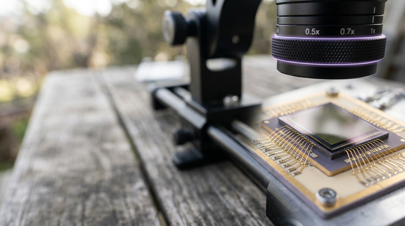
The event camera is worth a separate note because it drifts differently. Rather than sampling brightness at a fixed frame rate, an event camera reports a stream of asynchronous per-pixel brightness-change events, and the comprehensive survey of the field characterizes the resulting advantages — very high dynamic range, on the order of 140 decibels versus roughly 60 for a conventional sensor, microsecond-scale temporal resolution, and much lower data rate under static scenes — while also noting that per-pixel threshold mismatch and noise are intrinsic to the architecture and vary from pixel to pixel and over time [4]. For a power-constrained field deployment this is a genuine trade: an event sensor’s near-zero output under a static scene is a direct power win, since a conventional frame sensor spends the same read-out energy whether or not anything changed, but the per-pixel calibration burden shifts from “sample rate” to “threshold uniformity,” and that calibration itself has to be revisited periodically in the field rather than assumed to hold for the unit’s lifetime.
Privacy is an architecture decision, made once, at design time
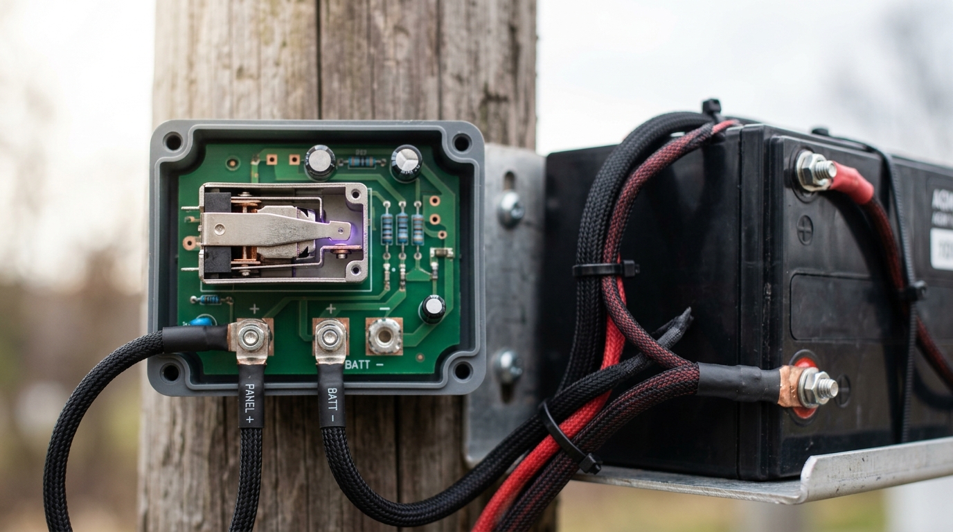
The privacy question in an edge AI sensor system is often framed as a policy question — what does the privacy notice say — when it is actually an architecture question decided when the data path is designed, long before any policy is written. The relevant design axis is simple to state and hard to execute: for each category of sensed data, does raw or lightly processed information ever leave the device, and if some aggregate does leave, what does the aggregation guarantee about what cannot be reconstructed from it.
The applied literature here is more mature than the framing above suggests. Apple’s published research on protecting private federated learning against reconstruction attacks is a useful primary source specifically because it is explicit about the threat model it defends against and the one it does not: the technique described adds a defense against an adversary that tries to recover individual training examples from an aggregated model update, on top of the differential-privacy noise already applied to that update, and the paper is candid that this is a targeted mitigation for a specific attack class rather than a general proof of privacy [7]. That specificity is the right register for describing any on-device privacy claim in a product: “raw audio never leaves the device” is a falsifiable, checkable architectural claim; “your data is private” is not, and a deployment document should prefer the former register throughout.
The practical design pattern that recurs across always-on audio and vision edge systems is a cascade with a hard boundary: an always-on stage (the sub-milliwatt keyword detector or coarse motion threshold discussed above) runs continuously and locally, and only its detection decision, not the raw sensor stream, is allowed to cross the boundary toward any further processing or network transmission. The keyword-spotting hardware literature already cited exists largely because of this boundary: a wake-word detector that ran in the cloud would require streaming raw audio continuously, which is both a power cost and a privacy exposure that the industry has specifically engineered around by pushing the always-on decision on-device [8] [10]. The same reasoning generalizes to vision and inertial sensing: an event camera’s native output is already a sparse change stream rather than a full image, which is a data-minimization property that falls out of the sensor’s physics rather than an added privacy feature, and a design that only forwards derived events, never accumulated frames, inherits that property directly [4].
Where this reasoning has to stop short of prediction is in the strength guarantees. It is defensible fact that a well-implemented on-device cascade reduces the volume and identifiability of data leaving a node. It is analysis that a differential-privacy mechanism, correctly configured, bounds what an observer of the aggregated output can infer about any one contributor’s raw data, with a quantified privacy budget stated in the mechanism’s own terms. It is a mistake — and one this article deliberately avoids — to describe any of this as making the system’s outputs “anonymous” or “impossible to trace,” categorical claims the underlying mechanisms do not make and their own authors do not make either.
The analog front end and the control loop it feeds
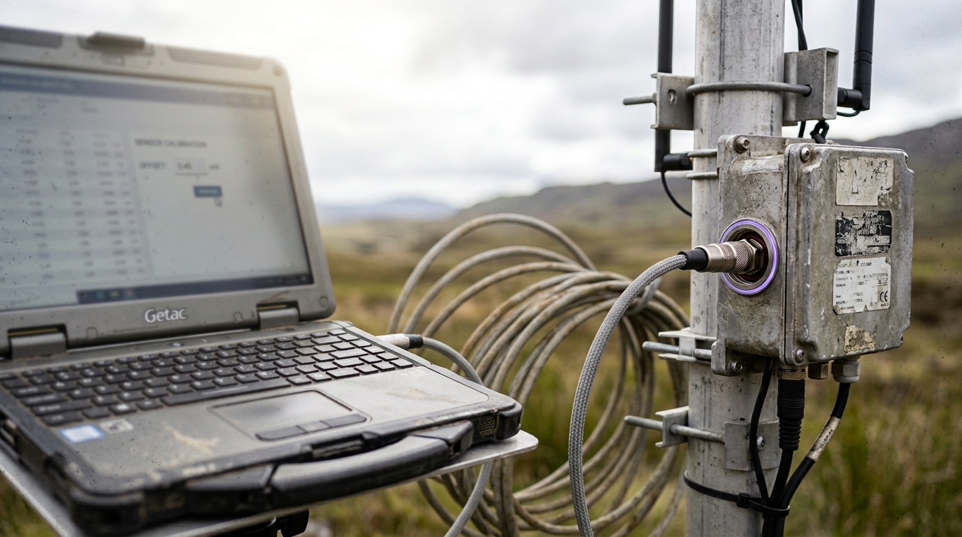
Every section above treats the sensed signal as though it arrives at the processor already clean, and it does not. Between a MEMS die or an event sensor and the inference model sits an analog front end — amplification, filtering, and an analog-to-digital converter — and that front end’s own imperfections compound with the drift discussed above rather than sitting apart from it. An ADC’s effective number of bits is not the number printed on its datasheet; it is a measured quantity that falls with quantization noise, thermal noise, and nonlinearity, and it is exactly why IEEE 1241 defines standardized terminology and test methods for characterizing analog-to-digital converters as a distinct discipline from the converter’s nominal resolution [9]. A twelve-bit converter operating with an effective number of bits closer to nine or ten because of front-end noise is a common, unglamorous field reality, and it directly narrows the dynamic range a drift-compensation routine has to work with: correcting a sensor offset in software is only as good as the quantization step that offset is measured against.
This is where “control” enters as its own concern rather than a synonym for inference. A field node’s escalation logic — deciding when to wake the expensive model, when to trigger a recalibration pass, when to throttle sensing rate to conserve a low battery — is a control system with its own stability properties, and a poorly tuned one oscillates: a threshold set too close to ambient noise causes repeated false escalations, which is exactly the power-budget failure mode identified earlier, where the dominant term in average power is how often the cheap stage escalates rather than how efficient the expensive stage is once triggered. Hysteresis in the wake threshold — requiring the triggering condition to clear by a margin before resetting, not merely to cross a single line — is a standard control-systems answer to that oscillation, and it is worth stating plainly as engineering judgment rather than as a citation: no single study in this article’s source list measures hysteresis margins for edge AI wake logic specifically, so the recommendation here is analysis, not a reported result.
What actually fails, and on what horizon
Pulling the three threads together into an operating picture: a field-grade edge AI sensor node’s power budget is dominated by how rarely its cheap monitoring stage escalates to full inference, not by how efficient that inference is once triggered; its drift is dominated by thermal history more than by elapsed calendar time, which means field temperature logging is a cheap and valuable addition to almost any deployment; and its privacy posture is set by where the raw-to-derived boundary is drawn in the data path, a decision made once at design time and not adjustable later by policy language alone.
One dated, falsifiable prediction follows from the drift evidence above. Given that the measured aging studies show MEMS offset drift is gradual, roughly linear at a given temperature, and correctable by recalibration rather than requiring part replacement [5] [6], a reasonable expectation over the next three to five years is that more field-deployed sensor nodes will ship with an on-device self-test or lightweight in-field recalibration routine triggered on a temperature-weighted schedule rather than a fixed calendar interval. The assumption underneath that prediction is that the aging mechanisms characterized in bench studies to date generalize to the specific part families used in low-cost field deployments, which have not individually been aged for a decade under field conditions. An observable indicator would be MEMS vendors publishing temperature-indexed drift specifications rather than a single worst-case number, the way HTOL-style accelerated testing already reports failure rates as a function of junction temperature [2]. The disconfirmation condition is equally concrete: if large-scale field telemetry from deployed sensor fleets over the next several years shows drift correlating poorly with temperature history relative to raw elapsed time, the temperature-weighted recalibration argument would be wrong and a simpler fixed-interval schedule would be the better engineering default after all.
No source consulted for this article was rejected outright; two vendor-style capacity-fade claims for lithium battery chemistry were considered and deliberately left uncited because they could not be traced to an independent measured study rather than a manufacturer application note, and the article says so directly above rather than citing them as fact.