Edge AI Electronics and Sensor Systems in Practice: Quantization, Power Budgets, and Sensor Front Ends

Four decisions, one bench

Almost every failed edge AI deployment fails at one of four decisions, and almost none of them fail because the model was not accurate enough in the lab. A vision model that scores well on a validation set is quantized down to a representation the target chip can actually execute, and the quantization step changes what it computes. A device that runs for an afternoon on a bench supply is asked to run for a year on a coin cell, and nobody wrote down where the milliwatts were actually going. A sensor is chosen because a similar part worked on a similar project, and the analog front end built around it turns out to be the actual bottleneck. And a system that worked in the office is shipped into a parking garage, a freezer, or a field, where temperature, vibration, and years of duty cycles surface failure modes the bring-up bench never exercised.

This article works through those four decisions in the order a team actually meets them: how a trained model becomes firmware through quantization and compilation, how a power budget is derived and then checked against measurement rather than assumption, how a sensor and its analog front end are selected against real resolution-power-bandwidth tradeoffs, and where privacy and reliability commitments are made or broken by the physical design rather than by a policy document. Each section leans on a specific, citable result rather than a general claim about “edge AI,” because the specific results are where the actual engineering constraints live.

Quantization and the optimization workflow, from a trained graph to an integer-only image

A model trained in 32-bit floating point does not run on a microcontroller with a few hundred kilobytes of RAM and no floating-point unit worth using for anything but the occasional scalar. The standard fix is quantization: representing weights and activations as low-bit integers, most commonly 8-bit, and executing the forward pass using integer arithmetic end to end. The scheme that made this practical for commodity hardware is an affine mapping between a real value and its stored integer,

where $r$ is the real-valued number, $q$ is the stored integer, $S > 0$ is a scale factor, and $Z$ is an integer zero-point chosen so that real zero maps exactly onto a representable integer — a detail that matters because operations like zero-padding and ReLU depend on zero being represented without rounding error. Jacob and colleagues showed that with this scheme, matrix multiplications and convolutions can be carried out using only integer arithmetic, with the more expensive floating-point rescaling deferred to a single fixed-point multiply per output, and reported close to a fourfold reduction in memory footprint against 32-bit floats with accuracy close to the unquantized model on standard image classification and detection benchmarks ^[1].

Two decisions follow from that scheme, and teams get the second one wrong more often than the first. The first is how to quantize: post-training quantization (PTQ) calibrates scales and zero-points from a small unlabeled sample of representative inputs and requires no retraining, while quantization-aware training (QAT) simulates the quantization error during training so the network learns weights that tolerate it. Nagel and colleagues’ survey of both families is blunt about the tradeoff: PTQ is a lightweight, push-button method that works well down to 8-bit and sometimes lower, but QAT is usually necessary to hold accuracy at more aggressive bit widths or on architectures sensitive to quantization noise, at the cost of needing labeled data and a training pipeline the deployment team may not control ^[6]. The second, more commonly mishandled decision is what calibration data PTQ actually sees: a calibration set that is smaller, cleaner, or differently distributed than the deployed sensor’s real output produces scales that are technically valid and quietly wrong, and the failure does not show up until the device is already in the field.

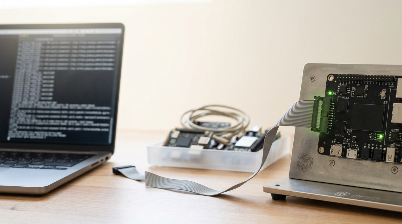
Quantization by itself does not produce a running device; the quantized graph still has to execute inside a tight interpreter or a compiled kernel library. TensorFlow Lite Micro takes the interpreter route deliberately, trading some per-op overhead for the ability to run the same op kernels across a fragmented landscape of Cortex-M and DSP targets without a separate compiled build per chip, and its authors are explicit that embedded targets sit one to three orders of magnitude below mobile phones in compute, memory, and power, which is what forces the framework to operate in tens of kilobytes rather than the megabytes a mobile runtime assumes ^[2]. CMSIS-NN takes the complementary route of hand-optimized, chip-aware kernels for Arm Cortex-M cores, reporting 4.6x throughput and 4.9x energy-efficiency improvements over baseline kernel implementations by using SIMD instructions where the core supports them and matrix-multiply-friendly data layouts ^[3]. In practice these are not competitors so much as different layers of the same stack: a framework decides how the graph is interpreted, and a kernel library decides how fast each op actually runs once it is called.

The most consequential move in this stack of the last several years has been to stop treating the network architecture as fixed and the deployment target as an afterthought, and instead search for both together. MCUNet pairs a neural architecture search restricted to a memory-and-latency budget (TinyNAS) with a code generator that produces a specialized inference engine for the chosen architecture rather than a general interpreter (TinyEngine), and the combination was the first system to cross 70% top-1 ImageNet accuracy on an off-the-shelf commercial microcontroller, doing so within a memory budget roughly 50,000 times smaller than a typical GPU training setup ^[5]. The lesson generalizes past that one result: on constrained hardware, the model and the runtime are not separable engineering problems, and optimizing one without the other leaves real headroom on the table.

Power budgeting: treating energy as a specification, not a hope

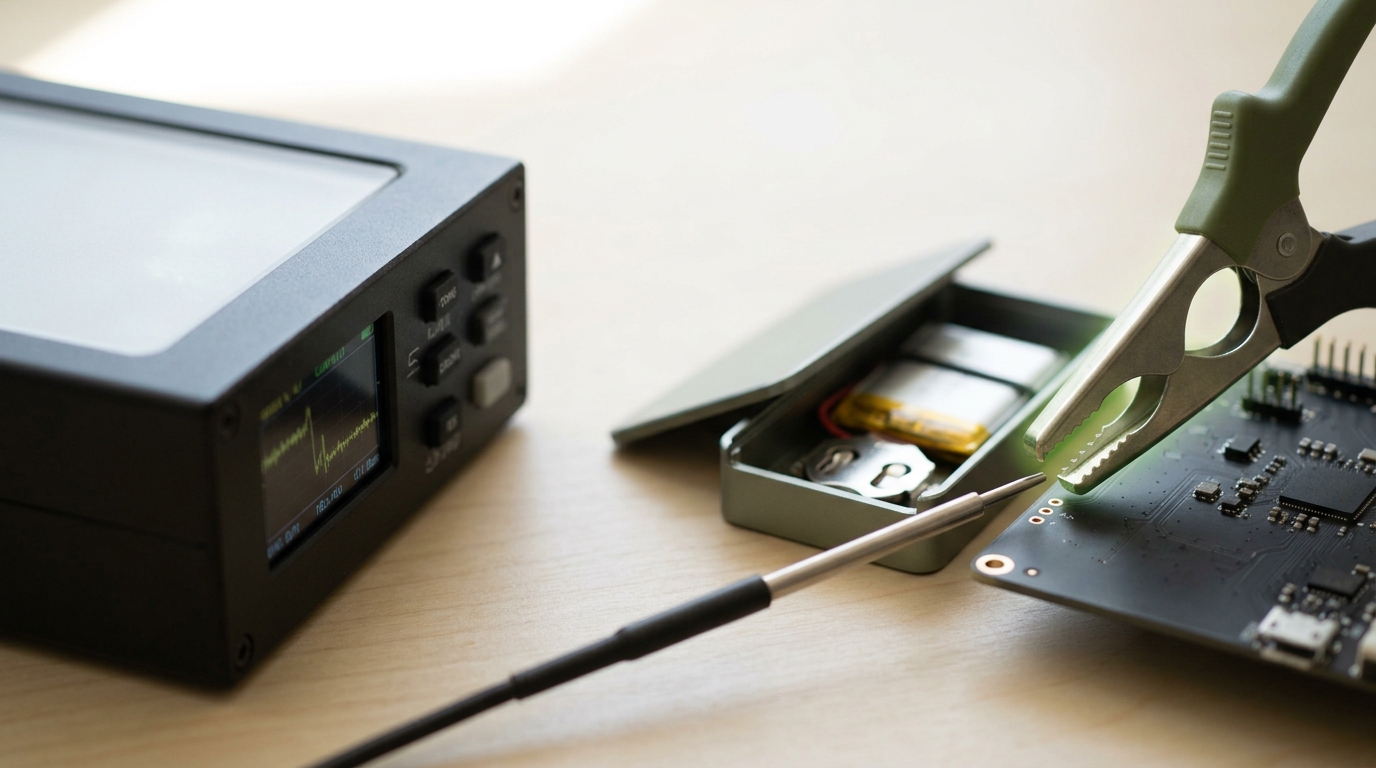
A power budget derived only from a datasheet’s typical operating current is a guess, and it is usually an optimistic one, because the datasheet number rarely includes the device’s actual duty cycle, its radio’s transmit spikes, or the current the sensor’s analog front end draws while settling before a reading is valid. The more defensible starting point is a duty-cycle energy model built from measured, not assumed, currents at each state:

where $E_{\mathrm{cycle}}$ is the energy spent in one full wake-sense-infer-sleep cycle, the first two terms are housekeeping power integrated over the time spent in each state, and $n_{\mathrm{inf}}$ inferences each cost a measured $E_{\mathrm{inf}}$. Every term in that expression should be a number taken off a current probe at the actual rail, not a value copied from a component’s datasheet, because sleep current in particular is notorious for being dominated not by the processor but by whichever peripheral, pull-up, or leakage path the design forgot to disable.

The value of measuring $E_{\mathrm{inf}}$ specifically, rather than folding it into a generic active-power number, is that inference energy is what a model and compiler choice can actually move, while sleep and housekeeping power are largely a board-design and component-selection problem. This is also where standardized measurement earns its keep: before MLPerf Tiny, TinyML hardware and software claims were close to impossible to compare, because there was no shared methodology for what to measure or how, and the working group behind it built a suite that reports latency and energy alongside accuracy across four representative workloads — keyword spotting, visual wake words, small-image classification, and anomaly detection — specifically so that a “faster” or “lower-power” claim means the same thing across vendors ^[4]. Before that benchmark existed, an earlier survey of the field had already flagged the underlying problem directly: the TinyML community lacked any widely accepted, reproducible benchmark, which meant published numbers were essentially incomparable across papers and product datasheets alike ^[8]. A team budgeting power today should treat any competitor’s headline energy-per-inference figure the same way that finding recommends treating any unstandardized number — as a claim tied to a specific harness and workload, not a portable constant.

The single largest lever most teams have over $E_{\mathrm{cycle}}$ is not the inference itself but how rarely it needs to run, which is why event-driven sensing — waking the system only when a sensor’s own front end detects a change worth acting on, rather than sampling and running inference on a fixed clock — routinely dominates every optimization applied to the model. That principle carries directly into the next section’s sensor discussion, because some sensor architectures build the event-driven property into the transducer itself rather than leaving it to software.

Sensor selection and the analog front end: the tradeoff that happens before the model ever runs

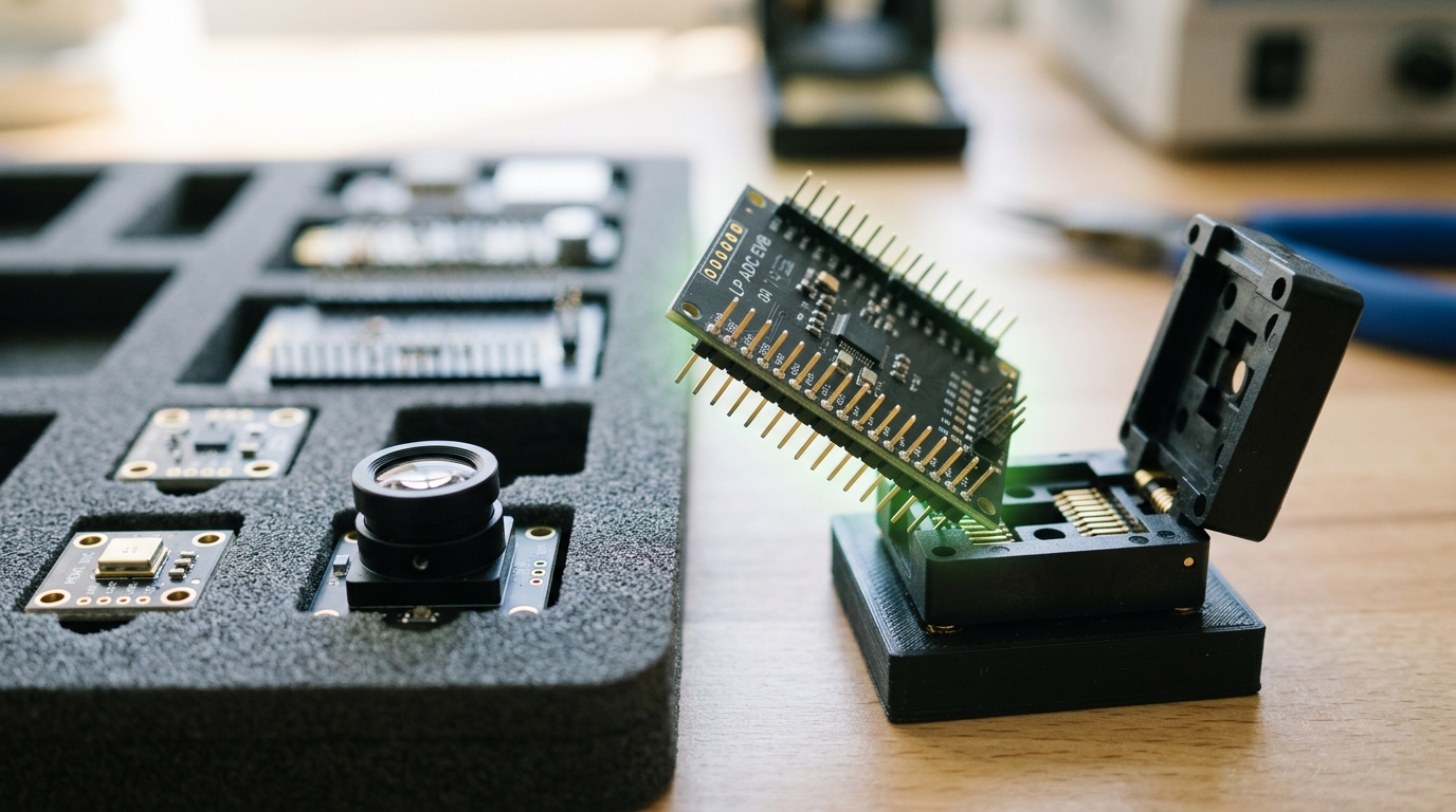
A model’s input quality has an upper bound set entirely by the analog front end that produced it, and no amount of downstream optimization recovers information the sensor and its converter never captured. The converter at the center of most low-power analog front ends is a successive-approximation-register (SAR) analog-to-digital converter, and a recent survey of low-power SAR design is useful precisely because it treats the tradeoff as an engineering surface rather than a single number: resolution, sampling speed, and power draw trade against one another through the comparator, the capacitive digital-to-analog converter, and the SAR logic individually, and pushing any one block toward lower power generally costs either speed, resolution, or both, with different mitigation techniques appropriate to each block ^[10]. The practical reading for a hardware selection meeting is that “low power ADC” is not a single spec to shop for; a part optimized for microwatt standby current at a few kilosamples per second is a different design, and a different tradeoff, from one optimized for the ten-to-twelve effective bits a vibration or audio front end actually needs.

Interchangeability across sensor front ends is itself a standards problem, not just a components one. The IEEE 1451 family of smart-transducer interface standards defines a common way for a sensor or actuator to describe itself to whatever processor or network it is attached to, through a Transducer Electronic Data Sheet carrying identification, calibration, and correction data alongside the raw measurement path, so that self-identification, self-description, and self-calibration are properties of the sensor rather than something a firmware team hand-codes per part number ^[9]. Designing toward that kind of standardized interface pays off specifically at the point a team wants to swap a sensor supplier or add a second source without re-deriving the analog front end from scratch — a real cost that is easy to discount during initial bring-up and expensive to pay later during a component shortage.

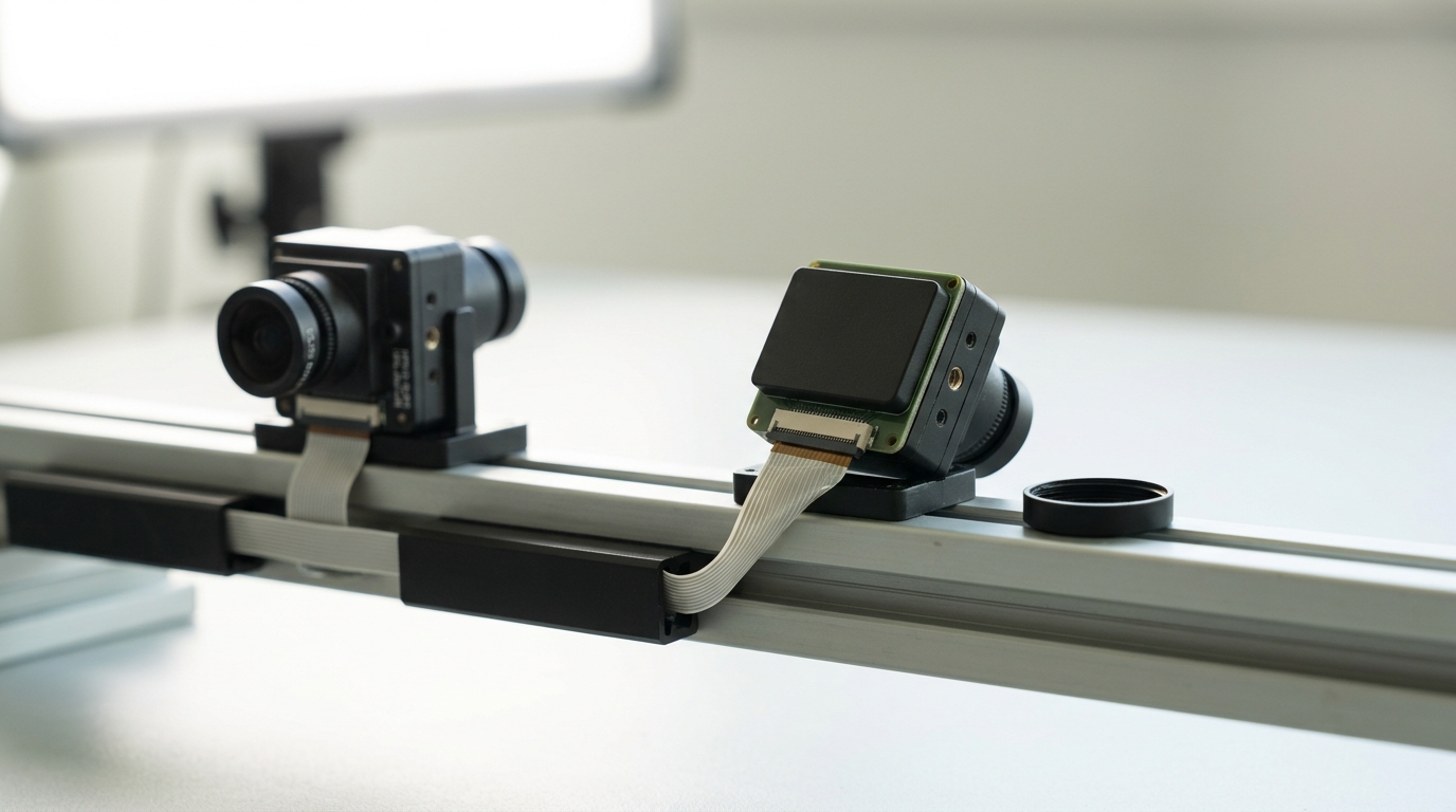
Vision front ends deserve separate treatment because the dominant architecture there is not a small variation on a conventional sensor but a genuinely different transducer principle. A conventional frame camera integrates every pixel over a fixed exposure and reads the whole array out on a clock, regardless of whether anything in the scene changed. An event camera instead reports, per pixel and asynchronously, only when the log-intensity at that pixel changes by more than a threshold, producing a sparse stream of timestamped events rather than a sequence of dense frames; Gallego and colleagues’ survey reports that this principle yields microsecond-scale temporal resolution, roughly 140 dB of dynamic range against the 60–70 dB typical of conventional sensors, and markedly lower power and data rate specifically because static scene content produces no events at all ^[7]. For an edge system whose energy budget is dominated by how often it has to move and process pixel data, an event camera turns “run inference less often” from a software policy into a property of the transducer itself — at the cost of a fundamentally different, and less mature, processing pipeline downstream, since the sparse, asynchronous event stream is not simply a smaller version of a frame.

Privacy at the edge: what leaves the device, and what an on-device model cannot promise

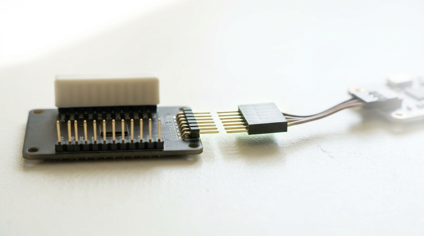
Running inference on the device rather than in the cloud is routinely presented as a privacy feature, and it is a real one for a specific, narrow reason: raw sensor data — an audio waveform, a full video frame, a continuous accelerometer trace — never has to leave the enclosure if only a classification result or a summary statistic is transmitted. That is a genuine reduction in what a network operator, a cloud provider, or an attacker on the wire can observe, and it is worth designing for explicitly, down to which physical connector or radio path a given signal is allowed to reach, rather than trusting that “the model runs locally” implies the raw data stays local too.

It is not, however, a complete privacy guarantee, and treating it as one is the mistake. A recent cross-paradigm survey of privacy-preserving machine learning for IoT is direct about this: an on-device model is still queryable, still has parameters that can memorize training examples, and remains vulnerable to membership-inference and model-inversion attacks that attempt to recover information about training data or infer sensitive attributes from the model’s outputs or even its power and timing side channels, so the survey treats differential privacy, federated learning, secure enclaves, and cryptographic approaches like homomorphic encryption and secure multiparty computation as complementary defenses against different threat models rather than a single solved problem ^[12]. Each of those defenses carries a cost that matters specifically on constrained hardware: differential privacy trades measurement accuracy for a formal noise guarantee, secure enclaves require silicon most microcontrollers do not have, and cryptographic approaches multiply compute and memory by factors that are often incompatible with a milliwatt power budget. The honest position for a design document is therefore to state which specific threat the local-inference design defends against — network eavesdropping on raw sensor data, typically — and which threats it does not, rather than letting “runs on-device” stand in as an unqualified privacy claim.

Common pitfalls when moving from lab to field

Four failure patterns account for a disproportionate share of the gap between a device that worked at bring-up and one that works a year into deployment.

Calibration data that does not match the deployed sensor. Post-training quantization scales are only as good as the sample used to derive them; a calibration set drawn from clean, curated inputs produces scales that clip or under-resolve the noisier, differently-biased signal a real sensor and its analog front end actually deliver in the field, and the resulting accuracy loss shows up as silent drift rather than a build failure.

Optimizing FLOPs while the actual constraint is memory. The MCUNet result exists specifically because standard neural architecture search targets accuracy per FLOP and treats memory as a soft constraint, when on a microcontroller peak activation memory is frequently the hard limit that determines whether a model runs at all, independent of how few multiply-accumulates it needs ^[5]. A model that is efficient by FLOP count can still fail to fit.

Trusting a lab-measured power number under a field duty cycle it was never tested against. The measurement discipline that MLPerf Tiny and its predecessor survey argue for exists because energy-per-inference numbers are tied to a specific harness, batch size, and clock configuration, and a number measured at bench temperature with a lab bench supply does not automatically transfer to a battery under a field’s real wake pattern, ambient temperature, and battery internal resistance at end of discharge ^{[4, 8]}.

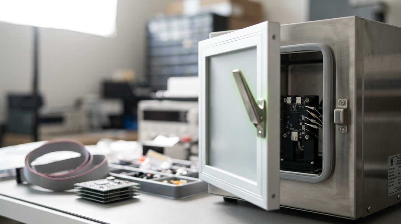
Aging effects that only appear after months of field time. Bias temperature instability, hot-carrier injection, time-dependent dielectric breakdown, and electromigration are all degradation mechanisms that shift transistor thresholds and interconnect resistance gradually under real operating stress, and a recent review of mitigation techniques for reliable integrated circuits treats in-field monitoring — voltage and timing margins tracked continuously rather than assumed constant from characterization — as increasingly necessary precisely because a part validated at time zero is not the same part a year into continuous field duty ^[11]. A device qualified only against a short burn-in at room temperature has not tested for this at all; the chamber exists to compress years of thermal and electrical stress into a schedule a team can actually observe before shipping.

Predictions, with the observations that would falsify them

These are forecasts, separated clearly from the sourced analysis above. Horizon: August 2029.

One. Architecture-search tools that jointly optimize a model against a named memory and energy budget, in the style MCUNet established, will become the default path for new microcontroller-class deployments rather than a research technique layered onto a hand-designed network after the fact. Disconfirmed if most production microcontroller deployments in 2029 still start from a manually adapted general-purpose architecture rather than a budget-constrained search.

Two. Standardized energy-and-accuracy reporting in the style of MLPerf Tiny will extend from a handful of reference workloads to being a routine line item in commercial edge-AI silicon datasheets, because the alternative — incomparable vendor-reported numbers — will have become commercially untenable as buyers get burned by transfer failures. Disconfirmed if leading edge-AI accelerator datasheets in 2029 still report accuracy and power on internally chosen, non-reproducible workloads with no standard reference point.

Three. Event-based and other sparse, asynchronous sensing front ends will spread beyond vision into other modalities — audio and vibration in particular — specifically because the event-driven property removes work at the transducer rather than in software. Disconfirmed if by 2029 event-driven front ends remain confined to vision applications with no comparable commercial adoption in audio or vibration sensing.

Four. In-field aging and margin monitoring, rather than fixed-schedule preventive replacement, will become standard practice for battery-powered devices deployed for multi-year lifetimes in variable thermal environments. Disconfirmed if multi-year field deployments in 2029 still rely predominantly on time-based replacement schedules with no on-device degradation telemetry.

None of these requires a discontinuity in the underlying physics or algorithms. Each follows from a pressure already visible in the sources above: measurement discipline replacing assumption, and the transducer itself increasingly doing work that used to be assigned to the model.

What to take away

None of the four decisions this article works through is solved once and then forgotten. A quantization scheme is only as good as the calibration data behind it; a power budget is only as trustworthy as the rail it was actually measured on; a sensor and its analog front end set a ceiling no model downstream can raise; and a device’s privacy and reliability properties are set by which wires and which stress mechanisms the physical design accounted for, not by a claim made about it afterward. Treat each of the four as a measurement to be repeated on the actual hardware, under the actual duty cycle, rather than a property inherited once from a datasheet or a paper, and most of the gap between a bench demonstration and a field-ready device closes on its own.