AI Memory Systems and the Bandwidth Wall in Practice: An Advanced Technical Guide

The number on the box and the number in the rack

Every team that serves a large model in production eventually has the same meeting: the accelerator’s datasheet promises one bandwidth figure, the model card promises one context length, and the node in the rack delivers neither at the same time. The gap is not a defect. It is the ordinary consequence of running a system whose dominant cost is moving bytes, under a workload — autoregressive generation — whose working set grows with every token it produces. Getting the delivered number close to the promised one is an operations discipline, not a purchasing decision, and it is learned at the level of the key-value cache, the batch, the kernel, and the memory tier, not at the level of the spec sheet.

This is a field guide to that discipline. It assumes the reader already knows why memory bandwidth binds before arithmetic does; it spends its words on what to actually do about it — which key-value cache strategy to reach for and when, how to size a batch against a memory budget instead of a compute budget, how to tell which roof a kernel is under before spending an afternoon tuning it, how to bring CXL capacity online without inheriting an unpleasant latency surprise, how to profile bandwidth utilization outside a lab, and where capacity plans most often go wrong. Facts here are attributed to the specific paper, standard, or vendor disclosure that reported them; where a number is a vendor’s own claim about its own product, it is marked as such rather than treated as an independent measurement.

Paging, evicting, and quantizing the key-value cache

The key-value cache is the part of a serving system’s memory footprint that a purchasing decision cannot fix, because it does not exist until a request is running. It grows with every generated token, in proportion to context length, batch size, layer count and head dimension, and its lifetime is exactly the lifetime of the request that owns it — arriving and departing unpredictably, at whatever size that request’s conversation happens to reach. A capacity plan sized for the average context length will be wrong for the tail, and a naive contiguous allocator sized for the tail will waste most of its memory on requests that never reach it.

with $L$↗ transformer layers, $H$↗ key-value heads, $d_h$↗ head dimension, $b$↗ batch size, $s$↗ sequence length and $p$↗ bytes per stored element, the factor of two counting keys and values separately. Every strategy below is, mechanically, an attempt to shrink one term of this product without shrinking the model’s effective context.

Paging attacks the allocator, not the product. Kwon and colleagues observed that existing serving systems store each request’s KV cache in one contiguous span of memory sized for its maximum possible length, and that this produces internal fragmentation, external fragmentation, and duplicated memory across parallel sampling requests — the paper reports that existing systems waste 60 to 80 percent of KV cache memory this way. Their PagedAttention design instead manages the cache in fixed-size blocks addressed indirectly, the same idea an operating system uses for virtual memory, and reports near-zero waste in KV cache memory alongside a 2 to 4 times improvement in serving throughput at the same level of latency compared with prior systems, with the improvement growing for longer sequences, larger models and more complex decoding algorithms ^[4]. Paging does not reduce $M_{\mathrm{KV}}$↗ per token; it reduces the waste around it, which in practice is often the larger number.

Eviction attacks $s$↗ directly by refusing to keep the whole history. The common pattern — a retained sliding window of recent tokens plus a small set of early “sink” tokens that attention disproportionately depends on — trades a bounded, workload-dependent quality cost for a hard, predictable ceiling on cache size regardless of how long a conversation runs. It is the right tool when a hard memory ceiling matters more than perfect recall of everything a request has ever said, and the wrong one when a downstream task genuinely depends on distant context; which regime a given product is in is an empirical question specific to that product’s workload, not a general property of eviction as a technique.

Quantization attacks $p$↗. Liu and colleagues’ KIVI method quantizes the key cache per-channel and the value cache per-token — an asymmetric scheme motivated by measuring that keys and values have different outlier structure, so a single uniform scheme for both leaves accuracy on the table. Their tuning-free 2-bit scheme is reported to hold quality nearly level with full precision across Llama-2, Falcon and Mistral while cutting peak memory, including model weights, by 2.6 times, enabling up to 4 times larger batch sizes and 2.35 to 3.47 times higher throughput on real workloads ^[5]. Those figures are specific to the models and workloads tested; a team adopting a cache quantization scheme should re-measure the accuracy cost on its own evaluation set before banking the memory savings, precisely because the asymmetry KIVI exploits was itself discovered by measurement rather than assumed in advance.

In practice these three are not alternatives; they compose. A production stack typically pages to eliminate allocator waste, quantizes to shrink the per-token footprint, and evicts only once a hard ceiling — set by capacity, by CXL tier latency, or by a service-level cost target — is actually reached.

Sizing the batch against the memory budget, not the compute budget

Batch size is usually taught as a throughput knob: bigger batches amortize fixed overheads and raise arithmetic intensity, so bigger is better until compute saturates. That framing is correct for prefill and actively misleading for decode. Prefill processes an entire prompt in parallel and is compute-bound; Pope and colleagues report 76 percent model FLOPS utilization during large-batch prefill of PaLM 540B ^[7]. Decode processes one token per request per step, re-reading the full weights and the entire accumulated KV cache from memory for each of those tokens, and is memory-bandwidth bound; the same paper reports 29 milliseconds per generated token with int8 weight quantization — a number set by bytes moved, not FLOPs issued. A batch-size decision made by watching only prefill throughput will systematically overcommit decode’s memory budget.

The two terms interact because the KV cache and the batch draw on the same pool. Raising batch size raises $b$↗ in the capacity equation directly; every request added to a batch adds its own cache, and past some point the node runs out of room for cache before it runs out of arithmetic. Multi-query and grouped-query attention relieve this by shrinking $H$↗, the number of distinct key-value heads a token’s cache must store — Pope and colleagues report that the resulting smaller footprint enables scaling to context lengths up to 32 times longer at fixed memory ^[7], and the same shrinkage buys headroom for a larger batch instead, if that is the more valuable trade for a given service.

When the model plus its cache simply does not fit the accelerator’s memory at any batch size worth serving, batch size stops being a knob and becomes the output of a placement problem. Sheng and colleagues’ FlexGen frames exactly this case: given a fixed hardware budget spanning GPU, CPU and disk, it solves a linear program over where to place weights, activations and the KV cache across those tiers, jointly with the batch size, to maximize throughput under a latency constraint. Running OPT-175B on a single 16 GB GPU, the reported configuration reaches an effective batch size of 144 and a generation throughput of 1 token per second — the first time, per the authors, that scale of model had been run at usable throughput on that little GPU memory — using 4-bit compression of both weights and cache to make the placement fit at all ^[6]. That is a boundary case, not a recommended steady-state configuration, but it demonstrates the general principle cleanly: once memory is the binding constraint, the batch size that maximizes throughput is whatever the placement solver says it is, not the largest number that technically executes.

The field diagnostic is simple and worth running before any deeper profiling: change the batch size and watch what moves. If per-request latency holds steady and total throughput scales with batch size, the node still has memory headroom and compute is the limit. If per-request latency degrades as batch size rises with throughput flat or falling, the KV cache is now competing with itself for bandwidth, and the fix is one of the three cache strategies above, not a larger batch.

Telling a memory-bound kernel from a compute-bound one before you tune it

The single most expensive mistake in kernel-level memory tuning is optimizing the wrong roof. A kernel waiting on bytes gains nothing from more parallelism, better instruction scheduling, or a faster arithmetic unit; it gains only from moving fewer bytes or moving them faster. A kernel waiting on arithmetic gains nothing from a bigger cache or a smarter memory layout. Guessing which regime a kernel is in from its name — “attention,” “matmul,” “layernorm” — is unreliable, because the same operation crosses the boundary depending on sequence length, batch size, and precision.

The practical fix is to measure arithmetic intensity directly rather than infer it. NVIDIA’s Nsight Compute profiler reports this as a first-class artifact: its Speed of Light section gives the achieved percentage of peak throughput for the compute and memory subsystems side by side for a profiled kernel, and its roofline chart plots the kernel’s measured arithmetic intensity and achieved performance against both the compute-bound ceiling and the bandwidth-bound slope in one view, so which roof is binding is read off the chart rather than assumed ^[11]. Run against the prefill/decode split above, this is exactly the tool that would show prefill sitting near the compute roofline and decode sitting near the bandwidth one for the same model on the same hardware — the 76 percent MFU and 29 millisecond figures reported by Pope and colleagues are, in effect, that same measurement taken at the system level rather than the kernel level ^[7].

Two operational consequences follow. First, profile after every change that touches precision, batching or attention variant, not only once at deployment — grouped-query attention, cache quantization, and a batch-size change each move a kernel’s arithmetic intensity, and a kernel that was comfortably compute-bound at one setting can cross into memory-bound territory at another without any code change. Second, treat a “kernel not at expected throughput” ticket as two separate questions — is the achieved percentage of the correct roof low, or is the kernel under the wrong roof entirely — because the fixes for each are disjoint and effort spent on one does nothing for the other.

Staging CXL memory expansion on measured numbers, not datasheet peaks

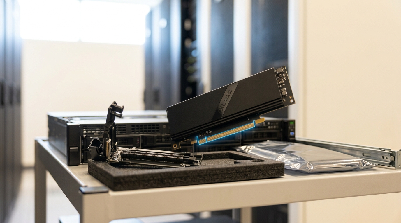
CXL memory expansion exists because HBM’s bandwidth comes bundled with a capacity ceiling set by package area and stack height. A single HBM3 device reaches up to 819 GB/s ^[3]; HBM4, standardized as JESD270-4 in 2025, doubles the independent channel count to 32 per stack and reaches up to 2 TB/s per stack in its base configuration, with higher configurations reported up to 3.3 TB/s ^[2]. Neither figure buys capacity beyond what fits on the package. CXL adds capacity by putting memory behind an interconnect instead of on the substrate, and the interconnect itself has kept scaling: the CXL Consortium’s 4.0 specification, released in November 2025, doubles per-lane transfer rate from 64 to 128 GT/s over the prior generation, adds bundled ports that let a host aggregate multiple device links for more bandwidth to one accelerator, and remains fully backward compatible with CXL 3.x, 2.0, 1.1 and 1.0, explicitly targeting AI and HPC memory pooling and sharing ^[1]. That is what the specification permits. What a deployed device actually delivers is a separate, and smaller, number.

Two independent measurement studies quantify the difference. Li and colleagues’ Pond, built on trace analysis of 158 workloads drawn from production Azure clusters, found that pooling memory across 8 to 16 sockets captures most of the achievable benefit, holding performance within 1 to 5 percent of same-NUMA-node allocation while cutting fleet DRAM cost by 7 percent ^[8] — a real, disclosed, and modest number, not the “half the DRAM for free” framing CXL pooling sometimes receives informally. Sun and colleagues went further and benchmarked genuine CXL-ready hardware rather than the emulated CXL that most earlier studies had relied on. Their pointer-chasing latency measurements found real CXL memory devices returning idle load latencies of roughly 155 to 360 nanoseconds against roughly 120 nanoseconds for local DDR5 — on the order of 1.3 to 3 times longer depending on the device — and sequential-read bandwidth efficiency of only 20 to 47 percent of theoretical peak across the three devices they tested, against 70 percent for local DRAM. They also report that genuine CXL hardware can show up to 26 percent lower latency than the emulated CXL setups used in prior literature, meaning results based on emulation should not be trusted for capacity planning in either direction ^[9]. A capacity plan that treats a CXL tier as DRAM with more room is planning against a device that, measured directly, is neither as fast nor as predictable as that assumption implies.

Placement policy recovers a meaningful share of what raw device latency costs. Sehgal and colleagues instrumented eight Micron CZ122 CXL E3.S devices added to a 128-core Intel Xeon 6900P system with twelve channels of DDR5-6400, configured as a unified NUMA domain with software-controlled page-level interleaving across local and CXL memory. Against a naive configuration, deliberate interleaving raised read-only bandwidth by 24 percent and mixed read/write bandwidth by up to 39 percent, for a 24 percent geometric-mean speedup across their combined HPC and AI workload suite ^[10]. The lesson generalizes past this one vendor’s parts: adding CXL capacity without an interleaving or tiering policy leaves a fixed, measurable fraction of the achievable bandwidth unclaimed, and that fraction is often larger than the gap between two competing devices.

The operating rule this supports: size CXL capacity for what the pooling literature actually reports — modest, fleet-level cost reduction at bounded pool sizes, not proportional capacity growth without bound — and budget its latency and bandwidth using measured device numbers from real hardware, not the specification’s ceiling or an emulator’s approximation of one.

Profiling memory bandwidth utilization in the field

Kernel-level roofline analysis answers whether one operation is under the right roof. It does not answer whether the memory subsystem as a whole — across local DRAM, CXL tiers, and whatever interleaving policy is active — is delivering what a workload needs under real, mixed, concurrent load, which is a different and equally necessary measurement. The methodology used by Sehgal and colleagues to characterize their Xeon 6 and CXL configuration is representative of what this looks like in practice: run bandwidth-scanning workloads across each memory tier independently and combined, under representative read/write mixes, before and after a configuration change, and report the achieved figure as a fraction of the theoretical one rather than the theoretical figure alone ^[10]. The same discipline applied at the kernel level, via a roofline-reporting profiler, and at the system level, via a tier-by-tier bandwidth scan, gives two independent readings that should agree; when they do not, the disagreement itself is diagnostic, usually pointing at an interleaving policy, a NUMA placement decision, or a driver default that neither measurement alone would have surfaced.

Three habits keep this measurement honest rather than decorative. Measure under the batch size and context-length distribution the service actually sees, not a synthetic best case — a bandwidth scan run at a single fixed batch size will miss exactly the regime change described in the batch-sizing section above. Re-measure after any change to precision, cache strategy, interleaving policy, or firmware, because each of those has been shown above to move the achieved fraction, sometimes by double digits, without moving the theoretical peak at all. And keep the measurement tied to a physical point in the system — a specific tier, a specific link, a specific kernel — rather than a single aggregate throughput number, because an aggregate can hold steady while the mix underneath it shifts from a cheap tier to an expensive one.

Where capacity plans actually go wrong

Most of the operational failures below are not exotic; they are the direct, predictable consequence of skipping one of the measurements described above.

Planning against a peak that was never achievable. A datasheet or specification ceiling — 819 GB/s per HBM3 stack, 128 GT/s per CXL 4.0 lane, 70 percent sequential-read efficiency even for local DDR5 — is a bound, not a forecast ^{[3, 1, 9]}. A plan built on the ceiling inherits a gap that measurement would have closed before deployment.

Sizing the KV cache for the average request instead of the tail. Paging exists because unmanaged allocators waste 60 to 80 percent of cache memory on exactly this mismatch ^[4]; a plan that assumes contiguous allocation at average length reproduces the failure mode paging was built to eliminate.

Treating a compression ratio as free. KIVI’s 2.6 times memory reduction and up to 4 times batch-size increase are measured results on specific model families, contingent on an asymmetric quantization scheme chosen because a naive one degraded quality ^[5]. A plan that assumes any cache quantization scheme yields the same ratio at no accuracy cost has skipped the step that made the reported ratio safe to ship.

Adding CXL capacity without an interleaving policy. Left at defaults, real CXL devices deliver a fraction of achievable bandwidth; deliberate page-level interleaving recovered 24 to 39 percent in one measured configuration ^[10]. Capacity that is present but not correctly placed does not show up as a fault — it shows up as unexplained latency that a capacity spreadsheet cannot see.

Assuming pooling benefits scale with pool size. Pond’s own data shows most of the achievable benefit captured at 8 to 16 sockets, with a 7 percent fleet-wide DRAM cost reduction as the headline result ^[8]. A plan that extrapolates linear savings from a larger pool is extrapolating past the point the underlying study actually measured.

Not re-measuring after a firmware, driver, or topology change. Every number cited in this article was obtained on a specific hardware and software configuration at a specific date. None of the papers above claim their measured figures transfer unchanged to a different device generation, and neither should a capacity plan.

Predictions, with the observations that would falsify them

These are forecasts, separated from the sourced analysis above. Horizon: 15 August 2029.

One. KV-cache quantization will become a default-on serving setting for long-context workloads rather than an opt-in optimization, because the KIVI-class evidence for near-lossless 2-bit quantization is now specific and reproducible enough for framework maintainers to trust as a default ^[5]. Disconfirmed if major open-source serving frameworks still ship full-precision KV cache as the unconfigured default for long-context deployments in 2029.

Two. CXL-tier interleaving and page-placement policy will move from a manual tuning step into an automated, workload-aware scheduler decision, because the bandwidth left on the table by static defaults — 24 to 39 percent in measured configurations — is too large to leave to manual configuration at fleet scale ^[10]. Disconfirmed if leading server operating systems still require manual, static interleaving configuration for CXL tiers with no adaptive placement option by the horizon date.

Three. Reported CXL memory benchmarks will increasingly specify genuine hardware rather than emulated CXL, because the measured gap between the two — up to 26 percent — is now large enough that reviewers and practitioners will treat emulation-only results as provisional ^[9]. Disconfirmed if peer-reviewed systems venues in 2029 continue to publish CXL performance claims based solely on emulated hardware without a caveat.

Four. Fleet-wide CXL memory pooling adoption will track Pond’s reported pool-size finding rather than grow toward larger shared pools, meaning most production deployments will cluster around 8-to-16-socket pools rather than rack- or row-scale pooling ^[8]. Disconfirmed if a majority of disclosed hyperscale CXL pooling deployments by 2029 report pool sizes materially larger than 16 sockets.

What to take away

None of the techniques above is a substitute for the others, and none of them is free. Paging removes waste that quantization cannot see; quantization removes bytes that paging cannot see; eviction sets a ceiling neither can. Batch size is a throughput knob only until the cache it feeds collides with the capacity that holds it, at which point it becomes a placement problem to be solved jointly with where the weights and cache actually live. A kernel is memory-bound or compute-bound as a measured fact about a specific configuration, not a property of its name, and that fact changes every time precision, batching or attention variant changes. CXL buys capacity at a latency and bandwidth cost that is real, measured, and worse than the specification’s ceiling, and a placement policy recovers a meaningful fraction of it back. Every number in a capacity plan is a claim about a specific piece of hardware on a specific date, and the only way to know whether it still holds is to measure it again.