Serving a Frontier Model: The KV Cache, Batching, and What a Token Actually Costs

The briefing in one paragraph

The price of a generated token is set by memory bandwidth, not by arithmetic. Producing one token from a large transformer requires streaming the model weights and the entire accumulated key–value cache out of memory and doing comparatively little work with them. Every serving technique that matters in production — batching, cache-shrinking attention variants, paged memory management, speculative decoding — exists to raise the amount of useful output extracted per byte read. Understanding that one constraint explains most of what looks arbitrary about how these systems are priced and configured.

Why decoding is bandwidth bound

A transformer decoder generates autoregressively: each new token attends over all previous positions ^[1]. To avoid recomputing the whole prefix at every step, implementations retain the per-layer key and value tensors for every past position. That is the key–value cache, and its size grows linearly with sequence length:

for $L$ layers, $n_{\mathrm{kv}}$ key–value heads, head dimension $d_{\mathrm{head}}$, sequence length $s$, batch size $b$, and $p$ bytes per element. The factor of two counts keys and values.

Now count the work. Generating a single token for a single request performs roughly $2N$ floating-point operations for $N$ parameters, while requiring that all $N$ parameters plus the request’s cache be read from memory. The arithmetic intensity — operations per byte moved — is therefore close to one, which is one to two orders of magnitude below the ratio at which modern accelerators become compute bound. The hardware trend has made this worse rather than better: Gholami and colleagues report that peak server FLOPS have scaled at roughly 3.0× every two years while DRAM and interconnect bandwidth have scaled at only about 1.6× and 1.4× respectively, and argue that memory has consequently become the dominant bottleneck for decoder inference ^[7].

Prefill behaves differently. Processing a long prompt handles many positions at once, so it is compute bound and scales with prompt length. This asymmetry is why input and output tokens are priced separately, and why a long prompt with a short answer has a completely different cost profile from a short prompt with a long answer.

Batching, and why it is nearly free

If reading the weights dominates and the weights are read once per step regardless of how many requests are in flight, then serving $b$ requests together costs barely more than serving one. Throughput rises almost linearly in $b$ until something else binds. Pope and colleagues set out this partitioning analysis for large transformers and showed how latency, throughput, and cost trade against one another under different sharding strategies ^[2].

What binds is memory, and specifically the cache. Weights are shared across the batch; the key–value cache is not. Each concurrent request carries its own, and each grows with every token it generates. Achievable batch size is therefore

which falls as contexts lengthen. This is the mechanism behind an effect users notice without explanation: long-context workloads cost disproportionately more, because they crowd out the concurrency that made short-context serving cheap.

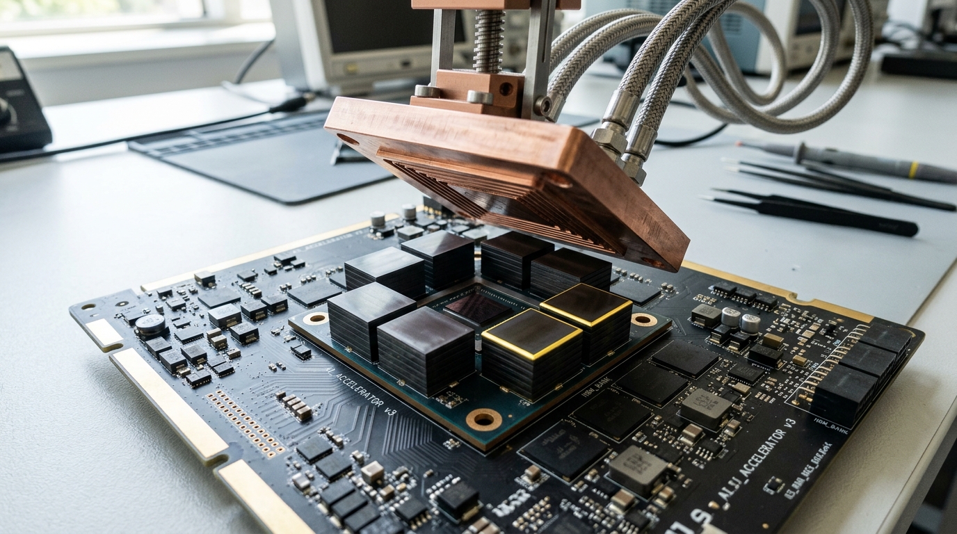
Kwon and colleagues attacked the denominator directly. Classical implementations reserve a contiguous block per request sized for the worst case, wasting most of it. PagedAttention borrows virtual-memory paging: the cache is stored in fixed-size non-contiguous blocks allocated on demand and shared across requests with common prefixes, which raises batch occupancy substantially at the same memory footprint ^[3].

Shrinking the cache at the architecture level

The other lever is $n_{\mathrm{kv}}$. Standard multi-head attention gives every query head its own key and value heads. Shazeer observed that the key and value projections could be shared across all query heads, cutting the cache by the head count at some quality cost ^[4]. Grouped-query attention interpolates: query heads are divided into groups, each sharing one key–value head, and the paper shows the resulting models can be uptrained from existing multi-head checkpoints to reach quality close to the original at speed close to multi-query ^[5].

This is a design-time decision baked into the weights, and it is the reason a model’s cost profile cannot be inferred from its parameter count alone. Two models of identical size can differ severalfold in achievable concurrency.

Speculation, and the distinction that matters most

Speculative decoding uses a small draft model to propose several tokens, which the target model verifies in one parallel pass; accepted tokens are kept and the first rejection is resampled. Leviathan and colleagues proved the construction leaves the target model’s output distribution unchanged ^[6].

That guarantee is the important part, and it draws the line a buyer should care about. Speculative decoding, paged memory, and batching change cost while provably or structurally preserving what is served. Quantisation, cache eviction, and prompt truncation change what is served. Both appear externally as a cheaper or faster endpoint. Only the second requires re-evaluation of your own workload.

Current OpenAI documentation exposes the caller-side half of this picture rather than the serving internals: as verified on 8 August 2026, the model guidance lists a family of gpt-5.6 variants at different capability–cost points together with a reasoning_effort control taking values from none to max ^[8]. How many tokens a given effort level produces is a property of the model’s post-training; what those tokens cost to emit is a property of the serving stack. Neither is disclosed, and they move independently.

What to ask before trusting a price

• What is the output-to-input token ratio for my workload? Prefill and decode have different cost structures; a single blended price hides which one you are buying.
• How long are my contexts, in practice? Cost per token is a function of concurrency, and concurrency falls as contexts grow.
• Did a price change come with a behaviour change? Re-run a fixed evaluation set across the change and compare distributions, not headline accuracy.
• Is the endpoint pinned? An unpinned alias can move to a different family member, a different effort default, or a different serving stack, none of which is a code change on your side.

The underlying discipline is simple. Treat cost per token as an emergent property of a model, a workload, and a serving system observed on a particular date — never as a number attached to a name.