Dense, Sparse, and Distilled: Comparing Approaches to Frontier Model Capacity

The question these approaches are actually answering

“How do we make the model better” is not one question. A laboratory training a frontier system, a provider serving it at volume, and an engineer deploying it on constrained hardware face three different optimisation problems, and the methods that dominate discussion are answers to different ones.

Fix the vocabulary first. Let $N$ be total parameters, $N_a$ the parameters actually used to process a given token, $D$ training tokens, and $M$ the memory that must be resident to serve. For the dense decoder-only transformer that remains the default architecture ^[1], $N_a = N$ and $M \propto N$. Every method below breaks one of those two identities, and which one it breaks determines what it is good for.

Dense scaling, and the allocation that was wrong

The dense route is the baseline: more parameters, more data, more compute, with $C \approx 6ND$. Kaplan and colleagues established that loss falls as a power law in each of these over many orders of magnitude ^[2], and the field spent several years reading that as a mandate to grow $N$.

Hoffmann and colleagues showed the allocation had been wrong. At fixed training compute, parameters and training tokens should be scaled in roughly equal proportion, and the large models of that era were substantially undertrained for their size ^[3]. The correction was worth a great deal of quality at no extra training cost.

The important caveat for anyone serving a model is that compute-optimal training optimises the wrong objective. It minimises loss for a fixed training budget. A deployed system minimises the sum of training and inference cost, and when the request count is large the inference term dominates. Every parameter removed is paid back on every request forever, which is why a rational provider deliberately overtrains smaller models past the compute-optimal point. The dense route therefore does not have one answer; it has a family of answers indexed by how many requests you expect to serve.

What dense scaling breaks: nothing. It is the reference case, and its problem is precisely that $M$ and $N_a$ both grow with $N$.

Sparse routing: many parameters, few used

Mixture-of-experts breaks the identity $N_a = N$. Shazeer and colleagues introduced the sparsely-gated MoE layer, in which a learned gate selects a small subset of expert sub-networks per example, allowing parameter counts far beyond what could be densely activated at the same compute ^[4]. Fedus, Zoph, and Shazeer simplified it decisively: the Switch layer routes each token to exactly one expert rather than the top-$k$, which reduced routing computation and communication cost while preserving quality, and they scaled the approach to trillion-parameter models ^[5].

The economics are attractive and frequently overstated. Training compute scales with $N_a$, not $N$, so a sparse model can hold far more knowledge for the same training FLOPs. Patterson and colleagues, computing energy and carbon for several large models including Switch Transformer and GPT-3, found that large but sparsely activated networks can consume less than one tenth the energy of large dense networks without sacrificing accuracy ^[10].

What sparsity does not break is $M$. Every expert must be resident somewhere at serving time even though any given token touches one. Since decoding is bound by memory traffic rather than arithmetic — Gholami and colleagues report peak server FLOPS scaling at roughly 3.0× every two years against DRAM and interconnect bandwidth at about 1.6× and 1.4× ^[9] — a sparse model’s advantage is real in training and much more conditional in serving. It buys quality per training FLOP and per activated parameter; it does not buy memory.

Three failure modes are specific to routing. Load imbalance leaves some experts saturated and others idle, wasting the capacity that justified the design. Routing instability during training is the reason the technique took years to become practical. And expert specialisation is not controllable: which expert learns what is emergent, so a sparse model’s behaviour under distribution shift is harder to reason about than a dense model’s.

What sparse routing breaks: $N_a = N$. Best when training compute is the binding constraint and memory is not.

Distillation: cast the same pattern smaller

Distillation attacks $M$ directly. Hinton, Vinyals, and Dean set out the mechanism: train a small student to match the full output distribution of a large teacher rather than the hard labels, on the grounds that the teacher’s relative probabilities over incorrect classes carry information the labels do not ^[6]. The student learns a smoothed, information-rich target that is easier to fit than the raw task.

The modern version of this is central to how model families are constructed. The DeepSeek-R1 work is instructive because it reports both halves: reasoning behaviour induced in a large model through reinforcement learning on verifiable tasks, and that behaviour then transferred into smaller models ^[11]. This is now the standard shape of a product family — one expensive frontier training run, several cheaper students — and it explains why the small members of a generation improve in step with the large one rather than independently.

The trade is that distillation loses something and you do not get to choose what. A student matched to its teacher on aggregate benchmarks can diverge sharply on the tail: rare knowledge, unusual formats, adversarial robustness, long-horizon consistency. Aggregate parity is the easiest property to preserve and the least informative. Anyone adopting a distilled variant on the strength of a headline benchmark should test the specific tail behaviours their workload depends on, because that is exactly where the allowance was taken.

What distillation breaks: the link between capability and $N$. Best when serving memory or latency is the binding constraint and a teacher already exists.

Quantisation: fewer bits per parameter

The fourth route leaves the architecture alone and reduces the bytes each parameter occupies. Dettmers and colleagues showed this is not merely a matter of rounding. Beyond roughly 6.7 billion parameters, transformers develop systematic large-magnitude outlier features that appear across all layers and destroy naive quantisation precision. Their procedure isolates those outliers in higher precision while quantising the rest vector-wise, halving inference memory while retaining full-precision performance, and allowing a 175-billion-parameter checkpoint to be converted and used directly ^[7].

Quantisation is the cheapest of the four — no retraining, applied post hoc — which is exactly why it deserves the most scrutiny from a buyer. It changes the served function. Unlike speculative decoding, which provably preserves the output distribution, quantisation trades a distributional shift for memory, and the shift is small on average and not uniformly small. It concentrates where the outlier structure matters, which tends to be on precisely the harder inputs.

There is a related architectural lever that is decided at training time and behaves similarly: grouped-query attention reduces the key–value cache by sharing key and value heads across groups of query heads, and models can be uptrained from existing multi-head checkpoints to recover most of the quality ^[8]. This shrinks the per-request memory rather than the weights, which is what actually governs achievable concurrency.

What quantisation breaks: bytes per parameter, and quietly, the served distribution.

Comparing them on the axes that differ

Read down the memory column and the current landscape explains itself. Memory bandwidth is the binding constraint in serving, so the methods that reduce resident bytes — distillation, quantisation, cache-shrinking attention — are the ones that move price, while the method that reduces training cost — sparsity — moves what is feasible to build. They are complementary, not competing, and production systems use all four at once.

This is also why parameter count has become nearly useless as a public signal. A sparse model’s headline count describes memory, not compute. A dense count says nothing about precision or attention layout. Current provider documentation has stopped quoting sizes altogether and instead names capability–cost tiers: the model guidance verified on 8 August 2026 lists gpt-5.6-sol, gpt-5.6-terra, and gpt-5.6-luna positioned by frontier capability, balanced cost, and high-volume efficiency ^[12]. Whether the difference between those tiers is distillation, quantisation, sparsity, or all three is undisclosed, and from the outside their effects are only distinguishable by measurement.

What a real production family looks like

None of the four is used alone, and the interactions are where the interesting arithmetic lives.

Consider a provider building a three-tier family from one training programme. The frontier tier is a large model, plausibly sparse, trained once at enormous cost and served on the most capable hardware available. The middle tier is a dense student distilled from it, deliberately overtrained past the compute-optimal point because it will absorb the bulk of request volume. The efficient tier is that student again, further reduced and quantised, with an attention layout chosen for cache size rather than for quality.

Trace one design decision through that structure to see why the tiers behave as they do. Suppose the middle tier’s key–value cache is halved by moving from multi-head to grouped-query attention. Achievable batch size is roughly

so halving the denominator roughly doubles concurrency at a given context length, which roughly halves cost per request at fixed hardware. The quality cost of that change, per the uptraining results, is small and concentrated on tasks that stress long-range attention ^[8]. A buyer sees a price cut. What actually happened is a targeted quality trade whose effects appear on a specific class of input.

Now apply the same reasoning to the efficient tier’s quantisation. The memory halves again, concurrency roughly doubles again, and the served distribution shifts in a way concentrated on the outlier features that emerge at scale ^[7]. Compounded with the distillation allowance already taken, the efficient tier can be several times cheaper than the frontier tier while being materially different on hard inputs and nearly indistinguishable on easy ones. That is exactly the profile that makes aggregate benchmarks misleading: the cheap tier looks close, because most benchmark items are not hard.

The economics that decide the mix

Which combination a provider chooses is not primarily a research question. Write total lifetime cost as

with $Q$ requests over the model’s life. When $Q$ is small — a research artefact, an internal tool — the training term dominates and compute-optimal allocation is the right target. When $Q$ is very large, the second term dominates by orders of magnitude, and every technique that reduces $\bar{c}_{\mathrm{inf}}$ pays back continuously while every technique that reduces $C_{\mathrm{train}}$ pays back once.

This asymmetry explains an otherwise puzzling pattern: laboratories publish scaling results framed around training efficiency, while providers ship products optimised almost entirely for serving efficiency. Both are behaving rationally about different terms of the same expression. Sparsity is a training-term technique that happens to be neutral-to-negative on the serving term. Distillation and quantisation are serving-term techniques that cost extra in the training term. A provider running both is not hedging; it is optimising two terms with two different tools.

The energy accounting reflects the same split. Patterson and colleagues, computing energy and carbon for several large models, found that large but sparsely activated networks can consume under a tenth the energy of comparable dense networks without sacrificing accuracy ^[10] — a training-side result. The serving-side energy story is governed instead by bytes moved, which is why memory-reduction techniques dominate operational cost even where they do nothing for training.

What the literature does not settle

Three questions matter commercially and are genuinely open.

Where distillation loss lands. Students are validated on aggregate benchmarks, which are dominated by items where teacher and student agree. There is no established method for predicting which capabilities a given distillation will sacrifice, so the tail loss is discovered empirically, per workload, after adoption.

Whether sparse models degrade differently under shift. Expert specialisation is emergent rather than designed. An input distribution unlike the training mixture may route poorly, and the failure signature of bad routing — plausible output from the wrong specialists — is not obviously distinguishable from ordinary error. No public methodology settles this.

How much quantisation error compounds over a long trajectory. Single-response evaluations show small distributional shifts. An agentic system taking two hundred dependent actions applies that shift two hundred times, and whether the errors cancel or accumulate is not established. Given that reasoning-trained models generate substantially more tokens per task by design ^[11], this is not a marginal question.

How to choose

If you are training: the allocation question comes first, and the answer depends on expected serving volume rather than on the training budget alone. Sparsity is worth the engineering if training compute binds and you can afford the memory.

If you are serving: reduce resident bytes before anything else, in the order quantisation, cache layout, distillation, because that is increasing order of cost to adopt and increasing order of quality risk.

If you are buying: ignore parameter counts, ignore aggregate benchmarks for distilled variants, and test the tail. The cheap tier of a family is almost always a smaller casting from the same pattern, and the allowance was taken somewhere. Find out where before it finds you.

A concrete procedure for that last case, since it is the one most readers face. Assemble fifty items from your own workload that you consider genuinely hard — the ones a competent junior would get wrong — and fifty that are routine. Run both sets against the frontier tier and the cheap tier at matched effort, five runs each, and compare the two gaps rather than the two scores. If the routine gap is near zero and the hard gap is large, you are looking at a distillation or quantisation allowance, and the cheap tier will serve you well until your traffic mix shifts toward the tail. If both gaps are similar, the tiers differ by something more uniform and the cheaper one is a straightforward saving. This takes an afternoon and answers a question no published benchmark can.

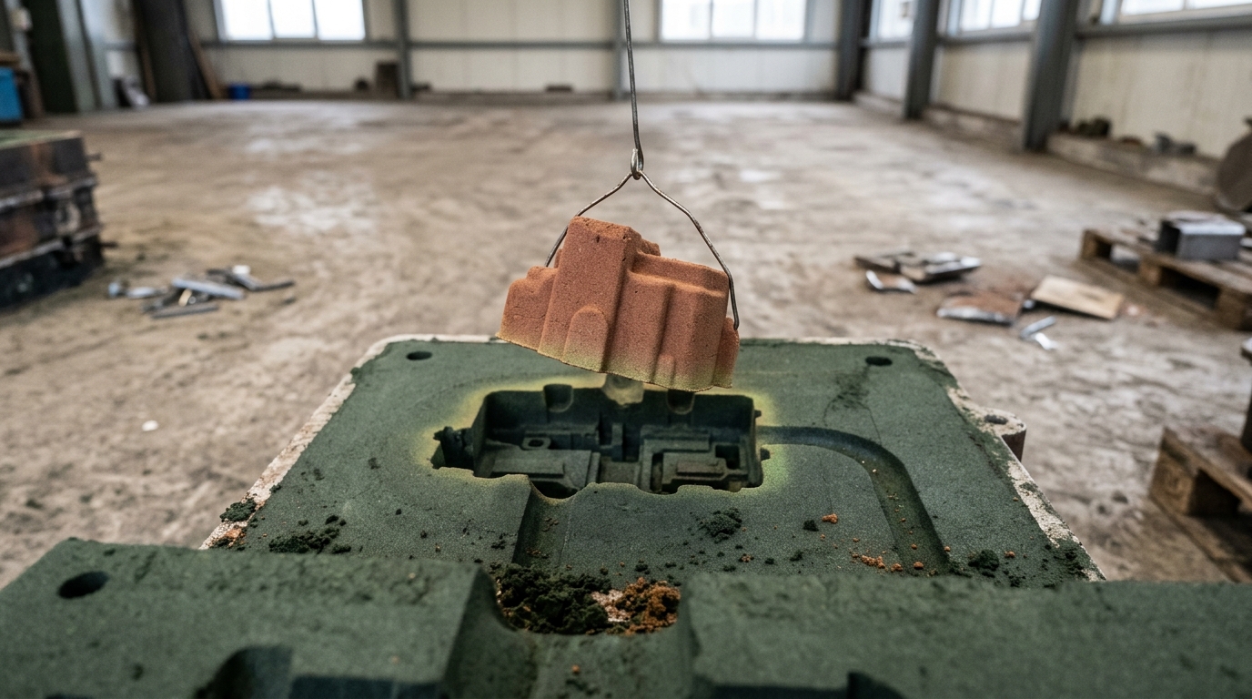
The pattern shop analogy holds to the end. Three moulding methods, one master pattern, three parts that measure alike on the drawing and behave differently in service. The drawing is the benchmark. Service is your workload.