The number in the slide deck is not the number in production
A team evaluates an accelerator, runs a benchmark, and gets a throughput figure worth putting in a slide deck. Six weeks later the same part, in their own rack, running their own workload, delivers a fraction of it. Nothing about this is unusual, and nothing about it is a defect in the hardware. It is the predictable gap between a number reached once, by someone who controlled every variable, and a number sustained continuously, by a team that controls fewer of them than they think.
Independent large-scale operators have put figures on that gap. SemiAnalysis, in an analysis of clusters built around roughly 100,000 NVIDIA H100 GPUs, reported that leading labs were achieving FP8 model FLOPs utilization (MFU) around 35% and FP16 MFU around 40% on trillion-parameter-class training runs — well below the accelerator’s advertised peak, and achieved only after deliberate topology and reliability engineering [7]. On the inference side, Pope and colleagues reported 76% MFU for large-batch input processing of a 540-billion-parameter model on TPU v4 hardware with int8 quantization, a figure that is high specifically because it comes from a purpose-built partitioning strategy for that exact model and batch shape, not from a default configuration [5]. Both numbers are real achievements and both are the result of specific, describable engineering work. The purpose of this article is to describe that work: choosing a precision format on purpose, writing and building kernels that actually use the hardware’s memory hierarchy, profiling well enough to know what is actually limiting a kernel, tuning the collectives that bind many devices into one job, planning capacity around a sustained number instead of a peak one, and recognizing the operational pitfalls that quietly separate a demo from a production system.
MLPerf exists because this gap is systemic enough to need an industry-wide answer. Reddi and colleagues built the MLPerf Inference benchmark specifically because “the myriad combinations of ML hardware and ML software make assessing ML-system performance in an architecture-neutral, representative, and reproducible manner” difficult, and its first submission round collected more than 600 reproducible measurements from 14 organizations across more than 30 different systems [3]. A methodology that elaborate, built by a consortium rather than one vendor, is itself evidence that a single headline number does not travel well between one deployment and the next. This article does not build a ranking between accelerators — that is exactly the comparison MLPerf’s rules exist to make fair, and doing it informally from vendor-reported numbers produces exactly the incomparable claims the benchmark was built to prevent. Instead it stays at the level every deployment shares regardless of vendor: the practices that determine how much of a part’s capability a given team actually gets to use.
Selecting a precision format on purpose
The first decision, and the one most often made by default rather than by analysis, is what numeric format the workload runs in. Modern accelerators support a stack of them — 32-bit and reduced-range 32-bit formats for full precision, 16-bit floating point for most training, and 8-bit floating point for both training and inference on recent hardware. The decision is not “use the narrowest format the hardware supports.” It is a workload-specific trade between dynamic range, mantissa precision, and the bytes moved per value, and getting it wrong produces failures that only show up well into a run.
NVIDIA’s Transformer Engine documentation is explicit about why an 8-bit format is not one format but two: E4M3, with four exponent bits and three mantissa bits, represents values up to roughly ±448 and is suited to weights and activations, which need a modest range but benefit from the extra mantissa bit; E5M2, with five exponent bits and two mantissa bits, represents values up to roughly ±57,344 and is suited to gradients, which are frequently far smaller or larger than weights and need the wider range more than they need mantissa precision [10]. A team that picks a single 8-bit format for an entire training step because “8-bit” sounded like one decision has already made a choice most vendor documentation warns against.
The practical selection process has three parts, and none of them is optional. First, decide per tensor category — weights, activations, gradients, optimizer state — rather than per model, because their statistical behavior differs enough that one format rarely serves all of them well. Second, calibrate on the workload’s own data distribution rather than a vendor’s published accuracy table, because outlier-heavy activations or gradient spikes specific to one architecture or one dataset are exactly what a generic accuracy claim will not have tested. Third, treat the choice as provisional until it has been validated against a fixed quality target, not merely “close” to a higher-precision baseline — this is the same discipline MLPerf’s training benchmark imposes formally, since its rules require a run to reach a defined target quality metric before its time is counted, precisely because “some optimizations that improve training throughput actually increase time to solution” if they are pushed past the point where the model still converges to the same result [4]. A precision format that trains faster but needs more steps, or that trains fast and diverges outright on a rare batch, has not actually won anything.
Kernel and compiler practices: fusion and tiling
A reference implementation of a model — the version a framework runs out of the box — is almost never the version that should ship to production on a given accelerator. Between the two sits a body of compiler and kernel work whose two central techniques are fusion and tiling, and both exist for the same underlying reason: an accelerator’s arithmetic units are usually not the scarce resource, and the goal of a well-written kernel is to do as much arithmetic as possible on data it already has on-chip before touching off-chip memory again.
Two research compiler stacks illustrate the two ends of how this is automated. TVM performs graph-level optimization — deciding which operators can be fused and in what order — and then operator-level optimization using a learned cost model to search the space of tiling and scheduling choices for a target device, and its authors report that the resulting code is competitive with vendor hand-tuned libraries across CPU, mobile GPU, and server GPU targets, while also supporting new accelerator backends such as FPGAs that lack a mature hand-tuned library at all [1]. Triton takes a narrower, more hands-on approach: it exposes a tile — a statically shaped multi-dimensional sub-array — as the basic unit a programmer writes against, with an LLVM-based compiler handling the low-level scheduling of that tile onto the hardware, specifically so that someone without deep CUDA experience can write a kernel that approaches the performance of one written by a specialist [2]. Different as they are, both systems automate the same manual practice: keep operands resident in fast on-chip memory for as many arithmetic operations as possible, and do not write an intermediate result back to slow memory only to read it straight back in for the next operator.
In practice this shows up as a short list of concrete moves. Fuse elementwise operations — activations, bias adds, normalization — into the matrix multiply or attention kernel that produces their input, rather than launching them as separate kernels each of which pays a full round trip to memory. Tile a matrix multiply or attention computation to the size of the on-chip memory available, so that a block of the operands is loaded once and reused across many multiply-accumulate steps rather than re-fetched. Avoid unnecessary kernel-launch overhead in tight loops — most consequentially in autoregressive decoding, where a naive implementation launches a full round of kernels per generated token and pays that overhead on every single one. None of these are exotic; they are the default output of a mature compiler stack when one is available, and the manual work a team signs up for whenever it is not.
Profiling: telling a memory-bound kernel from a compute-bound one
Fusion and tiling are moves in a specific direction — they exist to change whether a kernel is limited by arithmetic or by memory traffic — which means the first job of profiling is establishing which of those two regimes a given kernel is actually in before touching anything. Guessing wrong wastes engineering time on the wrong lever: adding arithmetic capability to a memory-bound kernel does nothing, and trying to reduce memory traffic in a kernel that is already compute-bound does nothing either.
NVIDIA’s Nsight Compute documentation builds its profiling workflow directly around this question, presenting a kernel’s achieved performance against two ceilings at once — a peak-arithmetic boundary and a memory-bandwidth boundary — with the profiled kernel plotted by its arithmetic intensity; a kernel that lands under the sloped bandwidth boundary is memory-bound, one that lands under the flat peak-performance boundary is compute-bound, and the point where the two boundaries cross is the ridge point that separates them, giving an engineer a direct visual answer to which regime a kernel is in and how far it sits from the relevant ceiling [8]. Google’s equivalent guidance for its TPU line puts the same discipline first as a matter of process rather than visualization: “your first step when troubleshooting TPU performance is to profile your model,” and its performance guide goes on to give shape-specific rules that exist only because getting them wrong silently leaves throughput on the table — batch sizes should be a multiple of 128 or 1,024 depending on the target, and matrix multiplication dimensions should be sized to the hardware’s matrix unit, 128×128 on TPU generations before v6e and 256×256 on v6e and Ironwood [11]. A kernel launched with a batch or tile shape that does not respect those boundaries is not merely a little slower; it can fail to engage the hardware’s matrix unit efficiently at all, which looks from the outside like a mysterious utilization ceiling rather than a shape mismatch.
The practitioner mistake this section exists to prevent is treating a single wall-clock throughput number as diagnosis. Two kernels can report the same tokens-per-second figure for entirely different reasons — one starved for bytes, one starved for arithmetic issue slots — and the fix for each is the opposite of the fix for the other. Profiling that only measures elapsed time answers “how much,” never “why,” and every optimization decision in the two prior sections depends on knowing which of the two questions is actually in play for the kernel in front of you.
Multi-device scaling and tuning the collectives
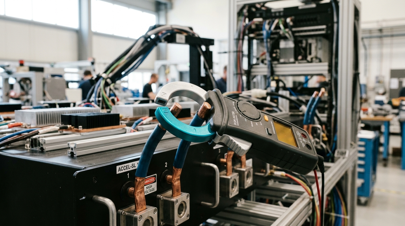
No single accelerator holds a frontier-scale model, so almost every production deployment is a multi-device job whose performance is bounded by the links between devices as much as by any one device’s arithmetic. The operations that run across those links are collectives — coordinated communication patterns among many participants at once, rather than a simple message from one device to another. NVIDIA’s NCCL documentation names the standard set: AllReduce, Broadcast, Reduce, AllGather, ReduceScatter, and AllToAll, alongside ordinary point-to-point send and receive [9]. Data-parallel training runs an AllReduce over gradients on every step; tensor-parallel execution inserts a reduction inside every layer’s forward and backward pass; mixture-of-experts routing is an AllToAll. These are not incidental background traffic — they sit on the critical path of every step a multi-device job takes, and a job cannot proceed past one until it completes.
Tuning them is a real, documented practice rather than a black box. NCCL’s environment-variable interface exposes algorithm selection through NCCL_ALGO, buffer sizing through NCCL_BUFFSIZE — 4 MiB by default — and topology-aware transport control through NCCL_P2P_LEVEL, which sets how close together two GPUs must be before NCCL will use a direct peer-to-peer path over NVLink or PCIe rather than routing through the host, alongside GPU-Direct RDMA controls that decide when a network adapter is judged close enough to a GPU to bypass host memory entirely [9]. Getting these defaults wrong on a given topology does not cause a job to fail; it causes it to run correctly and slowly, which is the harder failure to catch because nothing throws an error.
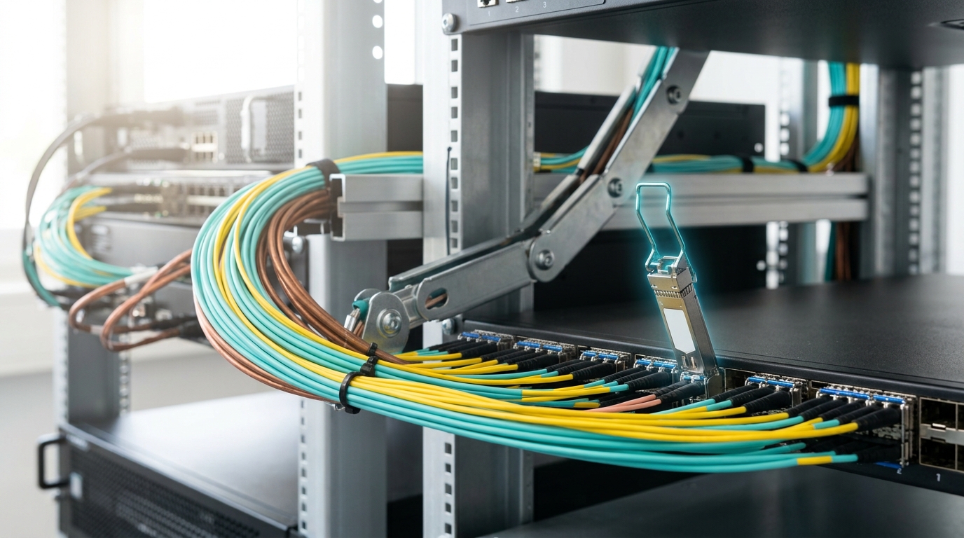
Topology itself is a first-class variable at cluster scale, not an afterthought layered on top of device count. SemiAnalysis’s account of 100,000-GPU H100 clusters describes network designs built around “islands” of full-bandwidth connectivity, with an oversubscription ratio — the piece cites a 7:1 example — applied between islands to control cost, and it frames the resulting Ethernet-versus-InfiniBand fabric choice as a genuinely contested one among operators rather than a settled question, since the two approaches trade differently on cost, congestion control maturity, and vendor lock-in [7]. That is a disagreement worth stating plainly rather than resolving: which fabric an operator should choose depends on scale, budget, and in-house networking expertise in ways that do not collapse to a single right answer, and any claim that one fabric is simply better should be read skeptically regardless of who is making it.
Capacity planning around a sustained number, not a peak one
Capacity planning built on a vendor’s peak specification, or even on a single well-tuned benchmark run, systematically overestimates what a production fleet delivers, because it leaves out two things that only show up at sustained, continuous operation: the utilization gap already discussed, and the fraction of wall-clock time the fleet is not running at all. A workable capacity model has to account for both. A simple way to state the assumption explicitly is
where
SemiAnalysis’s cluster-scale analysis makes the mechanism concrete: modeling a per-link mean time to failure of around five years across the very large number of transceivers and NICs present in a 100,000-GPU cluster, the piece estimates that a brand-new, fully working cluster would statistically see its first job-interrupting link failure within roughly half an hour of continuous operation, simply because of how many independently fragile links are running at once [7]. That is a modeled estimate from one operator’s analysis, not a universal constant, but the structural point generalizes: at sufficient device count, failure during a long job stops being an edge case to plan around and becomes the expected steady state to plan for. The same analysis distinguishes two recovery strategies with materially different costs — restarting from a saved checkpoint on disk, versus reconstructing lost state directly from the memory of surviving, healthy devices over the network — and reports the latter as meaningfully faster, describing it as capable of adding multiple percentage points back to sustained MFU on a large training run purely by shortening recovery time [7]. Capacity planning that only budgets for device count and ignores mean time to repair is budgeting for a fleet that does not experience its own failures, which no fleet at this scale actually is.
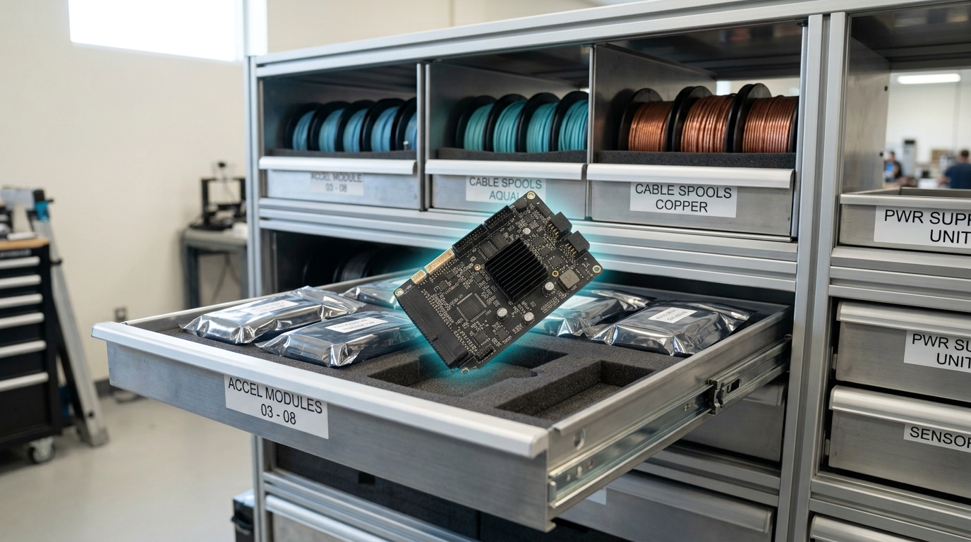
The staffing and inventory implication follows directly: staged spares reduce mean time to repair, and mean time to repair is exactly as load-bearing in the availability term
Where production throughput actually goes missing
The gap between a benchmark and a production fleet rarely traces back to one dramatic cause. It is usually several small, specific mismatches, each individually plausible and each individually a shortfall of a few percentage points, compounding.
Batch and sequence-length mismatch. A benchmark tuned at one batch size and sequence length, then deployed against production traffic with a different shape, silently leaves the matrix-unit and memory-hierarchy tuning described above misaligned with what the hardware actually sees — this is precisely why Google’s TPU guidance and MLPerf’s own scenario definitions are so specific about batch shape, since a number measured under one shape does not transfer to another [11] [3].
Host-side bottlenecks mistaken for device slowness. Data loading, preprocessing, and host-to-device transfer run on different hardware than the accelerator itself, and a starved accelerator waiting on the host looks identical from a coarse throughput dashboard to a genuinely compute- or memory-bound kernel. Profiling that stops at the device boundary, rather than tracing the whole pipeline, will misdiagnose this every time.
Firmware and driver skew across a heterogeneous fleet. A fleet built up over months rarely has identical firmware and driver versions on every node, and different versions can silently select different kernel implementations or collective algorithms for what looks like identical code — the diagnostics and validation workflow this article opens with exists specifically to catch that kind of divergence before it reaches production traffic.
Sustained-load thermal and power behavior. A short benchmark run can complete before a part’s thermal or power-limiting behavior under continuous load has fully engaged; a production job running for hours can throttle in ways a five-minute benchmark never observes.
Shared-cluster contention. On any multi-tenant cluster, network contention or scheduling interference from a neighboring job can look exactly like a compute problem from inside the affected job, and distinguishing the two requires instrumentation that spans the shared fabric, not just the local node.
Naive linear extrapolation from a single-node number. Multiplying one device’s throughput by device count ignores every collective-communication cost described above; Pope and colleagues’ own partitioning analysis exists precisely because the right multi-device strategy is workload- and topology-specific, not a constant multiplier applied to a single-chip number [5].
Measuring the average when the tail is what matters. For any accelerator fleet serving requests under a latency target, the number that determines whether the service level is met is not the median or the mean but the tail. Dean and Barroso’s foundational argument about large-scale systems is that “software techniques that tolerate latency variability are vital to building responsive large-scale” services, and that tail-tolerant design allows higher sustained utilization without sacrificing responsiveness — the opposite of the intuition that pushing utilization up necessarily makes tail latency worse [6]. A capacity or throughput report built entirely from averages is answering a question a latency-bound production service was never actually asking.
None of these pitfalls is exotic once named, and none requires new hardware to fix. They are, collectively, the specific difference between a number a team can put in a slide deck once and a number a fleet can sustain every day.
Predictions, with the observations that would falsify them
These are forecasts, separated explicitly from the sourced analysis above. Horizon: 15 August 2029.
One. Sustained, workload-measured MFU — rather than vendor-quoted peak FLOPS — will become the default unit that capacity planning and procurement are conducted in, as the gap between the two becomes too well documented to ignore. Disconfirmed if major cloud and cluster operators are still reporting capacity primarily in peak-FLOPS terms in 2029.
Two. Automated compiler-driven fusion and tiling (in the lineage of TVM and Triton) will account for a larger share of production kernel performance than hand-written kernels for new model architectures, because the manual-tuning cost of a new architecture will keep exceeding what teams can afford to redo by hand each generation. Disconfirmed if hand-authored kernels remain the dominant source of best-known performance for newly introduced architectures at that date.
Three. Availability-aware capacity planning — explicitly modeling mean time to failure and mean time to repair rather than assuming continuous uptime — will become standard practice at moderate cluster scale, not only at the frontier-scale clusters that currently publish this analysis. Disconfirmed if mid-sized deployments (low thousands of devices) still plan capacity from peak specifications with no explicit availability term in 2029.
Four. The choice between fabric technologies for multi-device scaling will remain a genuinely contested, context-dependent decision rather than converge on a single default, because the underlying trade-offs are structural rather than a temporary maturity gap. Disconfirmed if one fabric technology becomes the default choice across deployments of all scales and budgets by that date.
What to take away
A benchmark result and a production fleet are answering different questions. The benchmark asks what a system can do once, under conditions someone controlled deliberately. Production asks what a fleet does continuously, under conditions nobody fully controls — variable batch shapes, shared infrastructure, aging firmware, failing links, and a service-level target that cares about the tail rather than the average. Closing that gap is not one decision but five habits: choose a precision format for the specific tensors and workload in front of you, not by default; use or build kernels that keep data on-chip rather than trusting a reference implementation; profile well enough to know whether you are arithmetic-bound or memory-bound before you optimize either; treat multi-device collectives as a tuned, topology-aware system rather than a black box; and plan capacity from a sustained, availability-adjusted number rather than a peak one. None of this is exotic engineering. It is also, reliably, the entire distance between the number in the slide deck and the number the fleet actually delivers.