AI Inference Economics in Practice: An Advanced Technical Guide

Five levers, not one number

The economics of a token explain why a rate card looks the way it does: why input and output are priced differently, why a cached read costs a fraction of a fresh one, why a reasoning model can bill for text nobody sees. None of that explains what to configure on a Tuesday morning when the inference bill jumps forty percent overnight, or why a caching strategy that looked correct on paper produced a two percent hit rate in production. This article is the operational companion: a configuration guide for the decisions an engineering team actually makes, verified against primary documentation as it reads today rather than against how a feature was described at launch.

Five decisions determine most of what a production inference system spends, and none of them are visible on a pricing page. A caching strategy is a decision about how a prompt is assembled and how requests are ordered, made once in code and then either honoured or silently broken by the next unrelated change to a system prompt or a tool schema. A routing policy decides which requests reach the most expensive model, and on what evidence. A batching configuration trades latency for throughput, and the correct trade differs for a chat turn a user is watching and an evaluation job running overnight. A monitoring setup decides how many minutes of runaway spend a team tolerates before a human is paged. A procurement posture — on-demand, reserved, or self-hosted — is a bet on how confidently a team can predict its own utilization, because that confidence is the only thing that makes a commitment cheaper than paying as you go.

What follows works through each lever as currently documented by the providers who built it, verified independently rather than taken from secondary coverage, with two worked equations that turn “should we cache this” and “should we reserve this” into arithmetic a team can run on its own numbers.

Designing a caching strategy for a real hit rate

A cache-hit-rate target is either designed into a prompt or it is not achieved. Anthropic’s documentation is the most explicit of the three major providers about why targets are missed. A cache lookup on the Claude API walks backward from a declared breakpoint through a lookback window of at most twenty block positions; once twenty produce no match, the request writes a fresh cache instead of reading one ^[5]. The documented failure every team eventually reproduces: a system prompt with five stable blocks followed by a sixth carrying a per-request timestamp, breakpoint placed on that final block. Because the timestamp changes every request, the hash at block six changes every request, and the lookback walks back through blocks five through one without finding a match, since no entry was ever written there either — every request pays the write price, none pay the read price. The fix is to move the breakpoint to block five, the last block identical across requests, so the varying suffix sits after the cached region rather than inside it ^[5]. The rule generalizes: the breakpoint belongs on the last block that stays identical across requests meant to share a cache, never on one that changes every time — and Anthropic’s cache prefixes are built in a fixed hierarchy of tools, then system prompt, then messages, so a routine tool-schema edit invalidates a system prompt and history that never changed ^[5].

OpenAI enforces a version of the same discipline from the other direction: “a change before the breakpoint changes the prefix and will prevent a cache hit,” naming timestamps, tool definitions, schemas, message ordering, and image settings as the fields that commonly do this by accident when placed ahead of stable content ^[2]. Google states the identical principle from the caller’s side: put large, common content first, and send requests sharing a prefix close together in time, since implicit caching depends on temporal locality as well as textual identity ^[9]. Three independently engineered systems converge on one rule: static content first, in stable order, anything that varies pushed to the end.

Retention is the second lever, and here the platforms diverge. Anthropic prices two explicit windows — a five-minute write at 1.25 times base input and a one-hour write at 2 times — against a read price of 0.1 times base input in both cases, and states the multipliers stack with the Batch API discount and data-residency pricing ^[6]. OpenAI’s newest models offer less choice: on GPT-5.6 and later, a ttl parameter exists, but “the only supported value is 30m, which is also the default” ^[2] — the five-minute-versus-one-hour trade Anthropic exposes as a live choice is not yet available on OpenAI’s current generation, though earlier OpenAI models retain more variability, with default in-memory retention of five to ten minutes up to a one-hour maximum, or an extended mode reaching twenty-four hours ^[2]. A caching strategy has to be written per provider, because the retention knob it depends on may not exist on the platform it is ported to.

Google’s structure differs a third way: cached input prices at ten percent of standard input — verified today at 0.20 dollars against 2 dollars per million tokens for Gemini 3.1 Pro Preview — but a separate hourly storage fee is layered on top, charged whether or not the cache is read again ^[10]. Batching interacts with caching differently again here than on Anthropic: a cache hit inside a Google batch request bills at the standard cache rate rather than the batch-discounted one ^[8], while Anthropic’s pricing page states plainly that batch and caching discounts “can be combined” ^[6] — the same two features do not compound the same way on both platforms.

That convergence on roughly one tenth of base input for a cache read — independently verified today across all three platforms ^{[2, 6, 10]} — supports a design rule. Let $w$↗ be the write-price multiplier for the chosen retention window and $r \approx 0.1$↗ the read-price multiplier. For a prefix served identically $R$↗ times within that window — the first serving is the write, the remaining $R-1$↗ are reads — caching beats never caching once

is exceeded. At Anthropic’s five-minute rate, $w = 1.25$↗ and $R^{*} \approx 1.28$↗: the prefix pays for itself starting with the first read after the write, matching the break-even Anthropic’s pricing page states for that duration ^[6]. At the one-hour rate, $w = 2$↗ and $R^{*} \approx 2.11$↗, matching the stated two-read break-even for that window ^[6]. The formula’s use is computing the same threshold for a $w$↗ and $r$↗ that are not round numbers, and deciding, before writing code, whether a prefix’s expected reuse clears the bar for the TTL about to be selected.

Self-hosted systems face the inverse problem: not “will this prefix be read again” but “will the replica holding it be the one that receives the next matching request.” Mooncake, the serving platform Moonshot AI built for its Kimi models, addresses this by disaggregating the key-value cache from the accelerators that compute it, pooling underutilized CPU, DRAM, and SSD capacity across a cluster into a shared, addressable tier, and routing each request toward whichever node already holds the matching prefix — reporting, in vendor figures specific to that deployment, up to a 525 percent throughput increase in simulated long-context scenarios and 75 percent more requests handled in Kimi’s production service at the same hardware footprint ^[15]. A caching strategy that stops at prompt structure and ignores request-to-replica affinity has only solved half the problem a self-hosted fleet has.

Routing requests to a cost/quality tier

A router is a bet about which requests belong on an expensive model, and the two documented approaches differ in what evidence the bet is allowed to use. RouteLLM, presented at the 2025 International Conference on Learning Representations, trains a router directly on human preference data — pairs of responses from a strong and a weak model, labelled by which a human preferred — to teach a lightweight classifier when the weak model suffices ^[14]. The authors report the resulting router reduces cost by over two times in some cases while preserving quality, and that it transfers: swapping in a different strong or weak model pair after training does not require retraining from scratch ^[14], implying the router learns which prompts are hard rather than memorizing which model pair was used — a narrower, more defensible claim than “this router saves money,” worth verifying against a team’s own traffic before it is trusted.

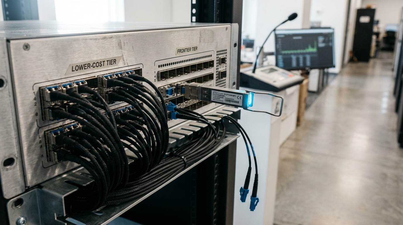
Amazon Bedrock’s Intelligent Prompt Routing is a live implementation of a similar idea. A router is built from exactly two models within one family; the caller sets a response quality difference threshold expressing how much better the non-fallback model’s predicted response needs to be before a request is sent to it instead of the fallback, and Bedrock predicts per request whether crossing that threshold is likely ^[12]. AWS states the benefit as optimizing “for both response quality and cost” — a vendor’s claim, worth distinguishing from an independently measured result ^[12]. The documentation is candid about limits worth repeating: routing “is only optimized for English prompts,” “can’t adjust routing decisions… based on application-specific performance data,” and “might not always provide the most optimal routing for unique or specialized use cases,” since effectiveness depends on the training data behind the default routers rather than a team’s own traffic ^[12]. As verified today, the default routers available during preview cover only Anthropic and Meta families, and the listed Claude models sit multiple generations behind the current line ^[12]: managed routing infrastructure has its own release cadence.

Two rules follow. A routing policy needs a fallback model chosen deliberately, not left as whatever is cheapest — Bedrock’s own criterion treats the fallback as the anchor a routing decision has to beat, so a badly chosen anchor biases every decision built on it ^[12]. And a router trained or tuned on someone else’s traffic should be validated against a held-out sample of a team’s own traffic before production use, precisely because both RouteLLM’s transfer result and Bedrock’s stated limits describe how well the routing generalizes, which only a team’s own prompts can answer; the tier boundary itself needs monitoring too, since a router whose tier mix drifts is either responding correctly to real traffic change or silently misrouting, and only tracking the mix over time distinguishes the two.

Splitting real-time and asynchronous traffic at the door

The most consequential batching decision is made at admission, before any serving-engine parameter matters: does this request need an answer now, or can it wait?

All three major providers price that answer explicitly. OpenAI’s Batch API discounts both input and output tokens 50 percent, completing “within 24 hours (and often more quickly),” and draws from a separate rate-limit pool that “will not consume tokens from your standard per-model rate limits” — up to 50,000 requests per batch, in a file up to 200 MB ^[1]. Anthropic’s Message Batches API offers the identical 50 percent discount, most batches finishing in under an hour with a 10,000-query ceiling, but a portability constraint worth checking first: batch processing is supported on the Claude API and Claude Platform on AWS, not currently on Amazon Bedrock, Google Cloud, or Microsoft Foundry ^[4]. Google’s Batch API matches the 50 percent figure and 24-hour target, and supports context caching inside a batch job — with the caveat already noted that a hit there bills at the standard, not batch-discounted, rate ^[8].

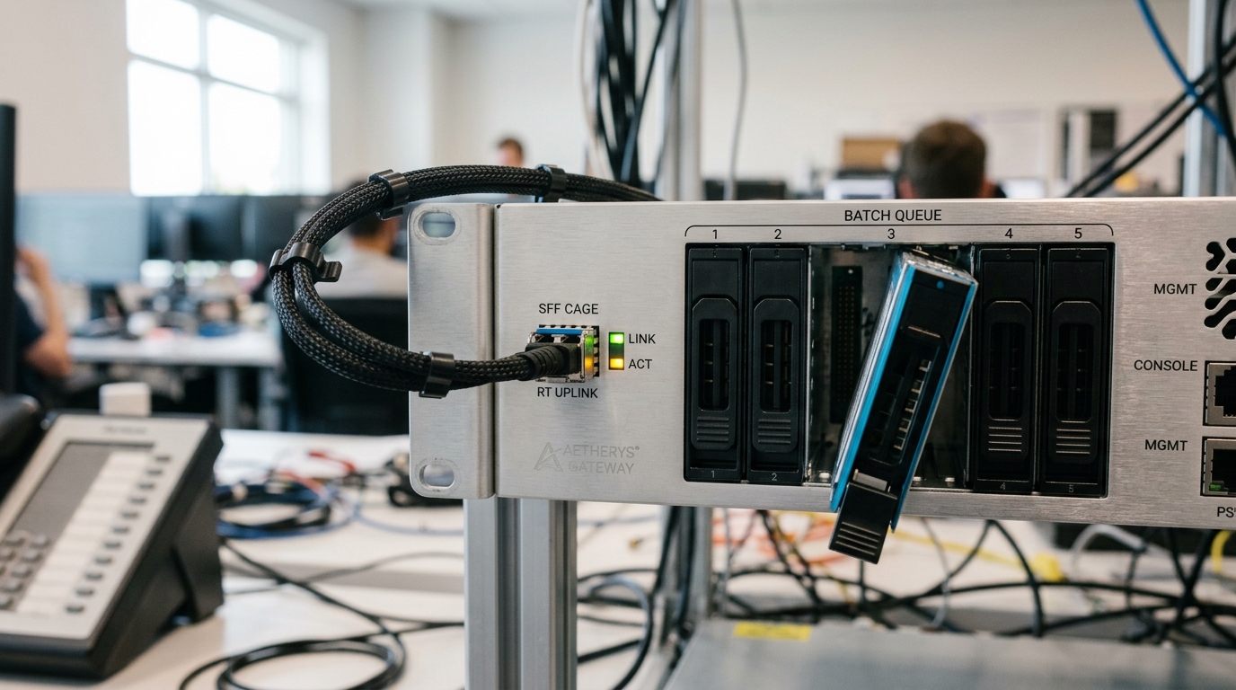
That is the easy half: anything genuinely deferrable — nightly evaluation runs, bulk content generation, offline extraction — belongs on batch, at no quality cost. The harder half is traffic that looks deferrable but is not quite: a triage queue that clears in minutes normally but backs up for hours during a spike, or an agent loop where some steps tolerate delay and others cannot.

The reason a real-time path and a batch path have to be engineered separately, rather than treated as one queue with a discount switch, is that they solve different scheduling problems. Orca, the serving system whose iteration-level scheduling underlies much of how modern engines batch real-time traffic, scheduled execution at the granularity of a single decoding step rather than a whole request, so a request finishing early returns immediately instead of waiting on its batch’s slowest member ^[16]. Evaluated against NVIDIA’s FasterTransformer on a 175-billion-parameter model, its authors report a 36.9 times throughput improvement at matched latency — specific to that model and hardware generation, not a general multiplier, but evidence that iteration-level scheduling makes a real-time path fundamentally different work from a batch file ^[16]. A batch endpoint optimizes total throughput over a bounded window with no per-request deadline; a real-time path optimizes the latency of the next token, continuously, for every request in flight — one system built to do both without configuring each path separately usually means each inherits the other’s worst property.

The practical rule is to classify traffic at ingestion, not after: interactive traffic goes to the real-time path regardless of load, and deferrable traffic goes to the batch queue regardless of how idle the real-time path looks, because the discount only applies to traffic actually submitted as a batch job. Overflow routing during a spike is a latency decision, covered next — conflating it with the sync/async split is the most common reason a batching strategy that looked correct in design saves less than the rate card promised.

Tuning the serving stack for your actual latency budget

For traffic staying on the real-time path, the batching decision moves from a discount toggle to continuous-batching parameters, and the correct values depend on which half of the latency budget matters more: time to first token, or time between subsequent tokens.

vLLM’s tuning documentation states this as a direct consequence of max_num_batched_tokens, which caps how many tokens the scheduler admits per engine step: smaller values “achieve better ITL [inter-token latency] because there are fewer prefills slowing down decodes,” while larger values “achieve better time to first token (TTFT)” ^[17]. The reason a long prefill slows decode at all is architectural: prefill is compute-bound and decode is memory-bandwidth-bound, so when both share one scheduling step, the prefill occupies compute other requests’ decode steps are waiting on. max_num_seqs — the ceiling on sequences resident in a batch — interacts with the same tradeoff from the concurrency side, and both are bounded jointly by the accelerator’s memory: max_num_seqs times maximum sequence length has to fit the KV-cache budget reserved via gpu_memory_utilization ^[17].

NVIDIA’s Triton Inference Server exposes a differently shaped version of the same knob: max_batch_size caps requests grouped into one batch, and max_queue_delay_microseconds sets how long the batcher waits for a batch to fill before sending an incomplete one — “the dynamic batcher will delay sending the batch as long as no request is delayed longer than the configured” value ^[18]. That single parameter is the entire latency-versus-throughput dial for a Triton deployment: near zero, every request dispatches quickly in small batches; extended, the batcher waits longer for company, at the direct cost of the delay added to every request.

Neither parameter set is right in the abstract — only right relative to a stated latency budget. An interactive interface has a TTFT budget in the low hundreds of milliseconds and tolerates a modestly higher ITL if the alternative is a visibly slow first token, governed by a queue-depth threshold rather than a fixed window. An agentic tool-calling loop often cares more about total trace time than any single token’s latency, and can tolerate a larger max_num_batched_tokens or longer queue delay for higher aggregate throughput across many concurrent sessions. One global batching configuration for both workloads is the most common way a serving stack ships with a latency SLA it cannot hold for one of its two traffic classes.

Mooncake’s scheduler shows the endpoint of this once a fleet needs automation: it implements a prediction-based early-rejection policy so an overloaded cluster refuses a request before committing resources rather than letting every in-flight request degrade together ^[15] — the principle a fixed queue-delay dial lacks by default, and the failure mode worth designing around before a genuine spike finds it first.

Cost monitoring and alerting that catches spend before it’s a crisis

The gap between an alert that prevents a crisis and one that documents it afterward is about what the alert is allowed to do, and providers draw that line differently. OpenAI separates two mechanisms easy to conflate. Spend alerts “send a notification; API traffic continues” — advisory only ^[3]. Hard spend limits, configured separately, “make API responses fail after the project reaches the limit,” returning 429 errors once crossed, with the guidance to “add alerts at thresholds that allow time to adjust usage, raise the limit, or investigate unexpected traffic” set below the hard limit so there is still room to act ^[3]. One caveat worth building into any hard-limit design: “enforcement is not instantaneous, so recorded spend can slightly exceed the configured amount” ^[3] — a hard limit bounds runaway spend, it does not guarantee an exact ceiling.

Anthropic structures this around workspace isolation instead: every organization has a default workspace and can create up to 100 more, each with independent spend limits that cap monthly spending and alert at chosen thresholds, and rate limits set per model tier — workspace limits may be set lower than the organization’s but never higher, so organization-wide limits always bind ^[7]. The practical value is attribution: separating environments or teams into workspaces gets per-workspace usage and cost reporting, the prerequisite for an alert to mean something specific rather than “aggregate spend moved,” a signal too coarse to act on quickly ^[7].

Both mechanisms are threshold-based, and a threshold only catches what it was set to catch: a cap sized from last month’s traffic says nothing about a gradual drift that never crosses the line until it is already large. AWS Cost Anomaly Detection targets that different failure mode — machine learning trained on an account’s own historical pattern flags deviations from the expected trajectory rather than a fixed number, running roughly three times daily with up to 24 hours of latency from the underlying billing data ^[13]. Its default threshold fires only when an anomaly exceeds both 40 percent of expected spend and a minimum 100 US dollars, and it returns up to ten contributing factors as a root-cause breakdown rather than one number ^[13]. No LLM provider reviewed here documents an equivalent layer of its own; provider-native spend limits alone leave a hard ceiling and a static warning, nothing that catches a slow-burning increase crossing neither line.

The FinOps Foundation names the structural reason static thresholds are harder to operate here than for most cloud costs: identifying “the consumer of the model output… is especially difficult when the consumers of the same model can be different” ^[19] — attribution has to happen before an alert can be routed to whoever can act on it, and that is frequently the missing piece rather than the alerting mechanism itself. Its recommended unit-economics metrics — cost per inference and cost per token, tracked per workload rather than blended — give an alert a denominator: a spend increase with proportionally more traffic is a growth signal; the same dollar increase with a flat request count is a regression, and only the ratio, not the total, tells them apart ^[19].

A layered design follows from stacking these rather than choosing one: a conservative workspace- or project-level alert, below a hard limit that exists purely as a backstop against a genuine runaway, anomaly detection running independently underneath both to catch drift that trips neither static threshold, and unit-economics tracking underneath all three to distinguish a real growth signal from a regression.

Forecasting budget from workload telemetry

A rate card prices one token. It says nothing about how many of each kind a workload will consume, and that gap is where budgets go wrong before they go wrong on the invoice.

The instrumentation this requires is specific: log five counts per request — new uncached input tokens, cache-write tokens, cache-read tokens, visible output tokens, and, on models that expose it, reasoning tokens billed at the output rate but absent from the visible response. A forecast built on one blended average collapses five quantities with different unit prices and different growth drivers into a number that moves for reasons a team cannot diagnose afterward. Decomposed, the same total spend increase reads differently depending on which count drove it: growth in cache-read tokens means the caching strategy above is working even as volume rises; growth in uncached new-input tokens means reuse is degrading.

The FinOps Foundation states the forecasting difficulty plainly rather than promising it away: for AI workloads, “predictability is generally lower” than for most cloud spend categories, calling for “more frequent revision of forecasts” as a structural feature of the category, not a sign of a badly built forecast ^[19]. That reframes what a forecasting process should produce — not a number holding for a quarter, but a live model rebuilt on a fixed cadence, with its own accuracy tracked.

Three practices follow. Segment before averaging: fit the five counts per identifiable request class — simple lookup, document analysis, multi-step agent trajectory — since a blended average describes no request actually sent, and classes typically differ in cache-hit ceiling and reasoning-token propensity. Track percentiles, not just means, since reasoning-token consumption is heavy-tailed and a mean-only forecast underestimates the tail driving peak spend. And price failure explicitly: a truncated request is billed in full and usually retried, so cost per accepted answer — total cost divided by first-attempt success rate — predicts budget more reliably than cost per request sent.

None of this needs exotic tooling. It needs the usage object every major provider already returns with each response to actually be logged, attributed to a workspace or project per the previous section, and rolled up on a cadence short enough that the forecast still describes current traffic rather than traffic from when it was last revised.

Procurement: on-demand, reserved, or self-hosted

Every major provider’s reserved-capacity product follows the same shape, and the shape is the procurement lesson before any specific number is.

Amazon Bedrock’s Provisioned Throughput sells dedicated capacity — measured in Model Units, each specifying input and output tokens processed per minute — billed hourly, for a commitment of no term, one month, or six months, with the discount increasing with commitment length ^[11]. The documentation is candid that the per-unit price is not published: “for more information about what an MU specifies, pricing per MU… contact your AWS account manager” ^[11]. That opacity is itself a procurement fact: a public formula cannot say whether reservation is worthwhile at a given volume, because the price half of the comparison is negotiated, not posted.

The arithmetic is simple once both prices are in hand, and generalizes across any reserved-capacity product structured this way. Let $P_r$↗ be the reserved capacity’s price per hour, $Q_{\max}$↗ the maximum throughput it sustains per hour at full utilization, and $c_{\mathrm{od}}$↗ the effective on-demand cost of the equivalent work. At actual utilization $u$↗, the effective cost per unit under reservation is $P_r / (u \, Q_{\max})$↗, and reservation wins exactly when

is cleared. Utilization above $u^*$↗ favours reservation; below it favours paying as you go. The formula’s value is what it forces a team to measure honestly before signing: not peak throughput or a favourable week’s average, but utilization sustained across the full commitment term including the slow periods — capacity sized to a launch-week peak and left running at a quarter of that traffic for the following eleven months has pre-paid idle time at the reserved rate.

This is where the earlier levers become procurement inputs rather than separate decisions. A caching strategy that lifts realized hit rate lowers $c_{\mathrm{od}}$↗, which raises the utilization bar $u^*$↗ a reservation has to clear — a workload with an excellent hit rate needs steadier, not just larger, volume to justify reserving, because caching already captured much of the available saving on-demand. A routing policy shrinking the volume on an expensive tier is a bet against reserving capacity for that same tier, and a batching strategy moving a large, predictable share of volume onto the batch discount changes what fraction of remaining traffic is even a candidate for a real-time reservation.

Self-hosting is the limiting case, where the commitment term is effectively indefinite and the fixed cost is capital and operating expense rather than an hourly rate — and it inherits the identical discipline. The serving-stack parameters covered earlier are the mechanism by which a fixed hardware footprint’s effective $Q_{\max}$↗ is set: vLLM’s guidance that gpu_memory_utilization, max_num_batched_tokens, and max_num_seqs are the highest-impact throughput knobs ^[17], and Mooncake’s demonstration that disaggregating the KV-cache tier can shift throughput by a reported multiple in specific scenarios ^[15], are the difference between a fleet’s real utilization ceiling and the number on a spec sheet. Evaluating self-hosting against a vendor’s on-demand rate without first establishing what the hardware can do compares a vendor’s optimized number against an unoptimized one, and will reliably conclude self-hosting costs more than it needs to.

The decision reduces to one variable in every case: how steady, and how confidently predictable, the utilization is. Bursty, hard-to-forecast traffic belongs on-demand, with caching and routing doing the cost work instead of a commitment. Traffic large and steady enough to forecast with real confidence, stable across a commitment’s full length rather than just at signing, is exactly the traffic a reservation — provider-managed or self-hosted — is priced to reward.

What to build first

The five levers do not need building in the order presented, and most teams lack the time to build all five before the next spend crisis. A rough priority, ranked by saving per unit of engineering effort in a typical workload: caching first, since a correctly placed breakpoint is a small change against an already-paid-for feature and the saving compounds on every hit. Monitoring second, since a layered alert is cheap to build and bounds the downside while everything else is tuned. Routing and the batching admission split third, together, since both classify traffic in a way that benefits the other. Serving-stack tuning and procurement last, since both depend on stable, well-understood traffic from the first four levers before there is anything reliable to tune or reserve against.

The throughline is what a pricing page cannot supply on its own: what a specific workload actually costs is a property of its own request shape, its own realized cache-hit rate, its own tier mix, and its own utilization curve — measured, not assumed, and re-measured on a cadence short enough to catch the next change before it appears as a surprise on an invoice instead of a line in a dashboard.