A number you can pace out
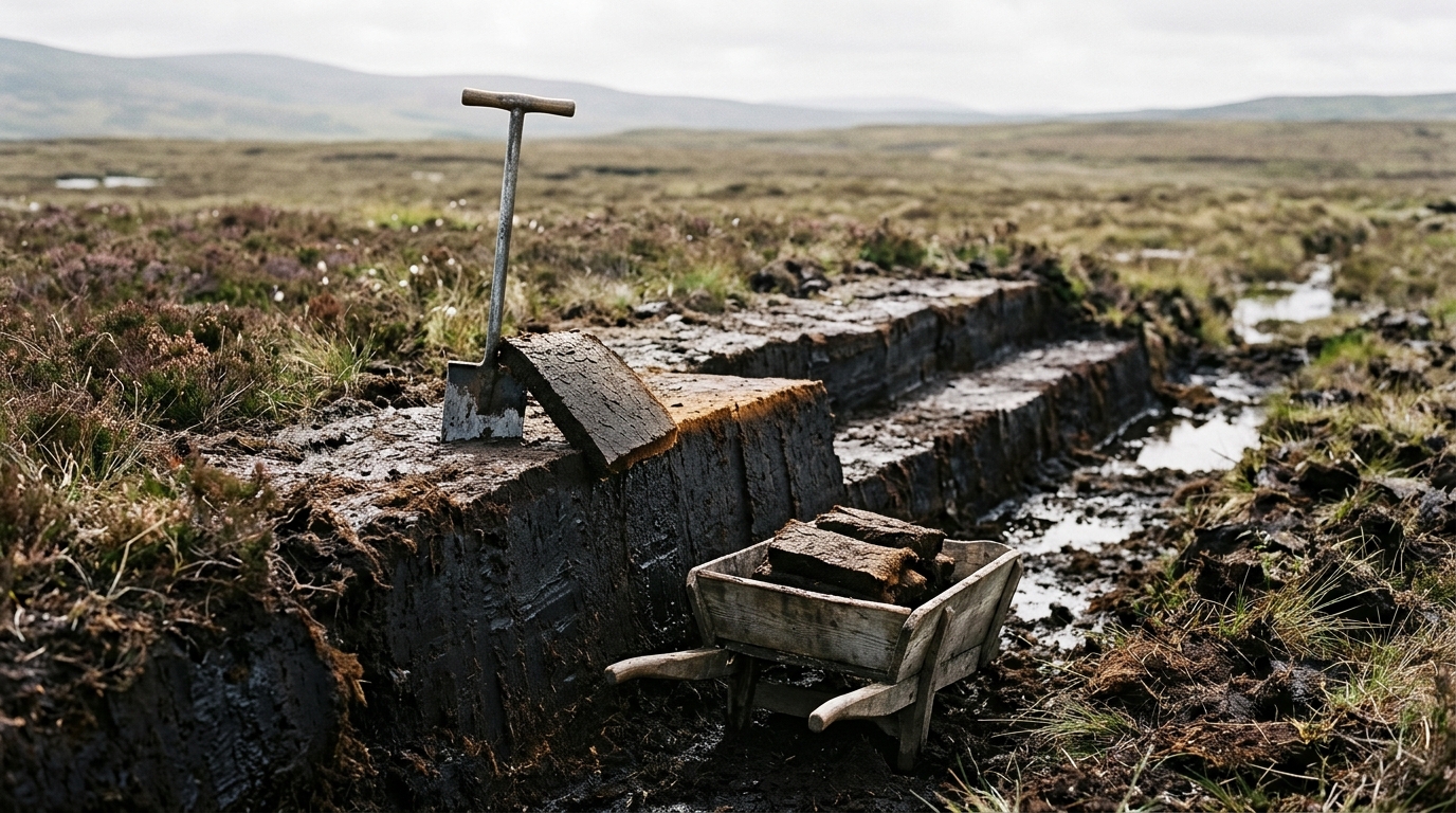
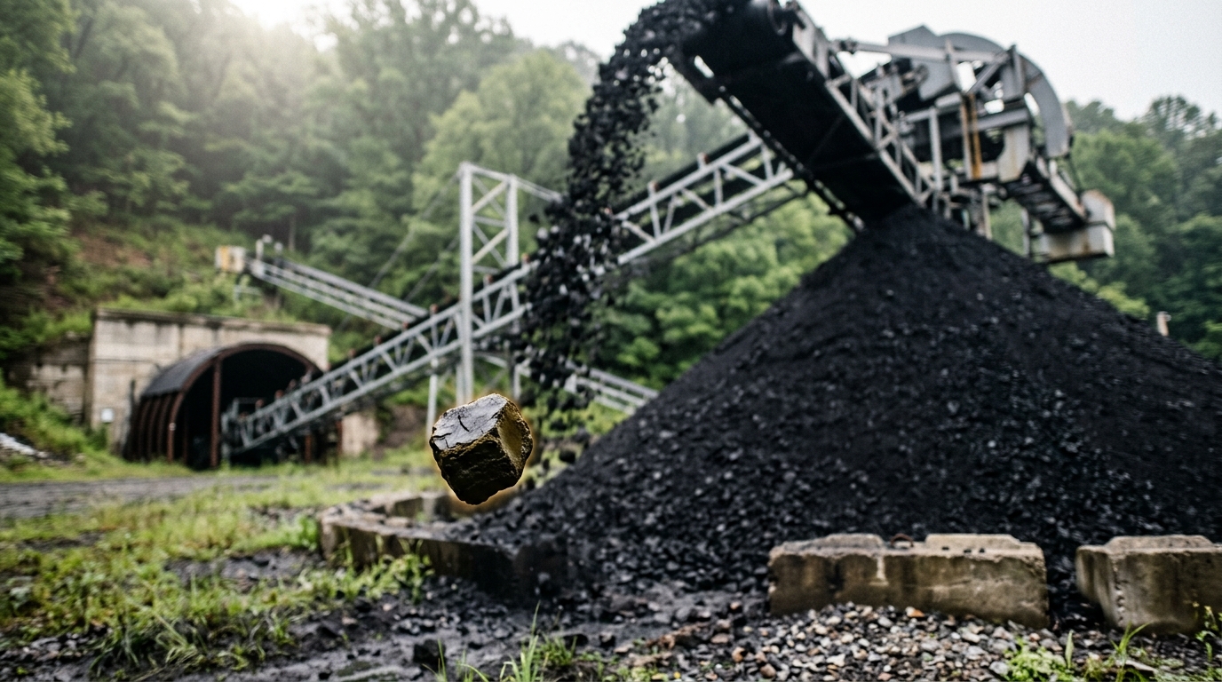
Almost every statistic in energy debate is an abstraction: a levelised cost, a tonne of carbon dioxide equivalent, a terawatt-hour. Power density is different. It is watts per square metre of horizontal ground, and it can be walked. Stand at a peat bank and the number is under your boots — so many square metres cut, dried, stacked and carried to heat one house through one winter. Stand at the head of a coal shaft and the same winter’s heat comes out of an opening you could park a cart on.
Vaclav Smil has been arguing for four decades that this comparison deserves to be a primary analytical variable rather than a curiosity. He is explicit that he chose an unusual definition. Engineers already used the phrase for antenna flux, for battery output per kilogram, for reactor core output per litre; the international system of units calls watts per square metre irradiance or heat flux density. Smil deliberately took a broader measure — “W/m2 of horizontal area of land or water surface rather than per unit of the working surface of a converter” — precisely because that version can be applied to everything from a wheat field to a gas turbine and so permits comparison across otherwise incommensurable systems [1]. His book-length treatment extends the same method to fossil extraction, thermal generation, renewable flows and end uses [2].
The metric is underused, and its critics have real objections. Both facts are worth taking seriously, and the order matters: understand what it measures before deciding what it settles.
Not energy density, not capacity factor
Two confusions do most of the damage.
The first is with energy density, which is energy per unit mass or volume. Smil notes the ordinary reasons this matters: air-dry wood reaches at best about 17 megajoules per kilogram, good bituminous coal 22 to 25, refined oil products around 42; natural gas at roughly 35 megajoules per cubic metre has a volumetric density about a thousandfold below crude oil’s 35 gigajoules per cubic metre, which is why gas moves by pipeline or as a liquid and oil moves in ordinary tankers [1].
Energy density and power density are independent. Troy Vettese, reviewing Smil’s book critically, gives the cleanest illustration of the split: charcoal and coal have very similar energy densities, since both are largely carbon, “yet the space required in their respective commodity chains is quite different, as the collier needs only a few hectares for a mine’s entrance and tailings, while a producer of charcoal needs massive tree plantations.” On Smil’s accounting, “coal has about five thousand times the power density of charcoal” [10]. The fuel in the hand is the same. The land behind it is not.
The second confusion is with capacity factor. Power density is an area-normalised output rate; capacity factor is a time-normalised one. They multiply rather than substitute. Writing energy generated as
The first factor, capacity density
Smil’s own wind numbers show the trap in miniature. Kinetic flux through the swept area of a rotor commonly exceeds 400 watts per square metre in the windiest mid-continental parts of America. Flux through the ground the farm occupies is a small fraction of that, because turbines must be spaced five to ten rotor diameters apart to limit wake interference [1]. Same technology, same wind, two legitimate square metres, two answers three orders of magnitude apart.
The span, with sources attached
Numbers repeated from memory are how this literature goes wrong. Here is what specific studies actually report.
Smil’s own summary table gives natural gas 200 to 2,000 watts per square metre, coal 100 to 1,000, photovoltaic solar 4 to 9, concentrating solar 4 to 10, wind 0.5 to 1.5, and biomass 0.5 to 0.6. His individual worked cases include the Olmedilla photovoltaic plant at about 9 watts per square metre of total site, Moura at 7.7, Waldpolenz at 4.1; Altamont Pass at 0.6 for wind, Puget Sound Energy’s Wild Horse at 2, and the London Array as designed at 1.44 [1].
Van Zalk and Behrens assembled 177 published density values across nine energy types and reported medians rather than ranges. Non-renewable systems came in at a median of 145.8 watts per square metre against 0.23 for renewables — a gap they characterise as more than three orders of magnitude. Within that: natural gas 482.1, nuclear 240.8, oil 194.6, coal 135.1; then solar 6.63, geothermal 2.24, wind 1.84, hydropower 0.14, and biomass lowest at 0.08 with a maximum across all biomass subtypes of only 0.60 [3].
Nøland and colleagues later analysed 870 plants across 32 countries using satellite imagery and site boundaries, and disagreed with parts of that picture. They report mean values of 764.69 watts per square metre for nuclear and 374.14 for natural gas — reversing the ranking — on the argument that van Zalk and Behrens charged natural gas with land from its whole value chain, of which pipelines account for roughly 80 per cent, while only about a third of natural gas use goes to electricity. Their renewable means are 20.33 for concentrating solar, 9.91 for photovoltaics, 4.88 for geothermal, 3.89 for offshore wind and 2.12 for onshore wind; hydropower’s mean of 33.73 carries a standard deviation of 157.28, which is a way of saying that hydropower has no characteristic power density at all, only a topography [8].
Two careful meta-analyses of the same concept, published four years apart, put nuclear and gas in opposite orders and disagree about photovoltaics by roughly 50 per cent. That is not a scandal. It is the metric behaving as a bookkeeping convention rather than a physical constant.
The area in the denominator is an argument
The clearest evidence for that reading is the wind dispute, which is worth following in full because it is unusually well documented.
Miller and Keith estimated wind power density from 411 US onshore installations and reported a 2016 mean of 0.50 watts per square metre [4]. They then published a corrigendum stating that “an error in the estimate of wind plant area led us to underestimate wind power densities by about 40%”, traced to “our incorrect specification of the geometric projection in the calculation of the area of Voroni polygons in our GIS software”. The corrected mean is 0.90 watts per square metre, with a 90th percentile of 1.48, and the authors maintain that “these corrections do not affect the overall conclusions of the paper” [5].
Mark Jacobson’s response objected not to the arithmetic but to the geometry. Assigning each turbine a polygon, he argued, “includes large amounts of space on the outside boundary of each wind farm… that is not actually occupied by a turbine”, allows overlapping notional areas, and ignores that real wind farms have irregular shapes and internal gaps between clusters. He illustrated with the Tule wind farm in California: a simple envelope around its 57 turbines implies 2.85 megawatts per square kilometre and about 0.86 watts per square metre of output, while tracing the ground actually around the turbines gives 29.0 megawatts per square kilometre and 8.7 watts per square metre [6].
Enevoldsen and Jacobson then formalised the alternative, applying a buffer equal to turbine tip height and connecting polygons only within clusters, across more than 1,600 operating turbines in 13 countries. European onshore farms come out at 19.8 megawatts per square kilometre installed and 6.64 watts per square metre output; non-European onshore at 20.5 and 6.84; European offshore at 7.2 and 2.94. Their own framing of the result is the important sentence: these are “substantially higher installed and output power densities than previously reported, based simply on different definitions of land area, with no impact on capacity factor” [7].
So the total area decomposes into parts that different analysts include or exclude:
A recent multi-method study makes the sensitivity explicit rather than arguing about it. Covey and colleagues measured 60 onshore and 24 offshore wind plants and 54 solar plants across six countries, computing capacity density four ways on the same plants. Onshore wind comes out at 4.9 megawatts per square kilometre by Voronoi polygon, 6.2 by five-diameter buffer, 4.0 by eight-diameter buffer and 4.4 by convex hull [9]. The plants did not change. The choice of boundary moved the answer by more than half.
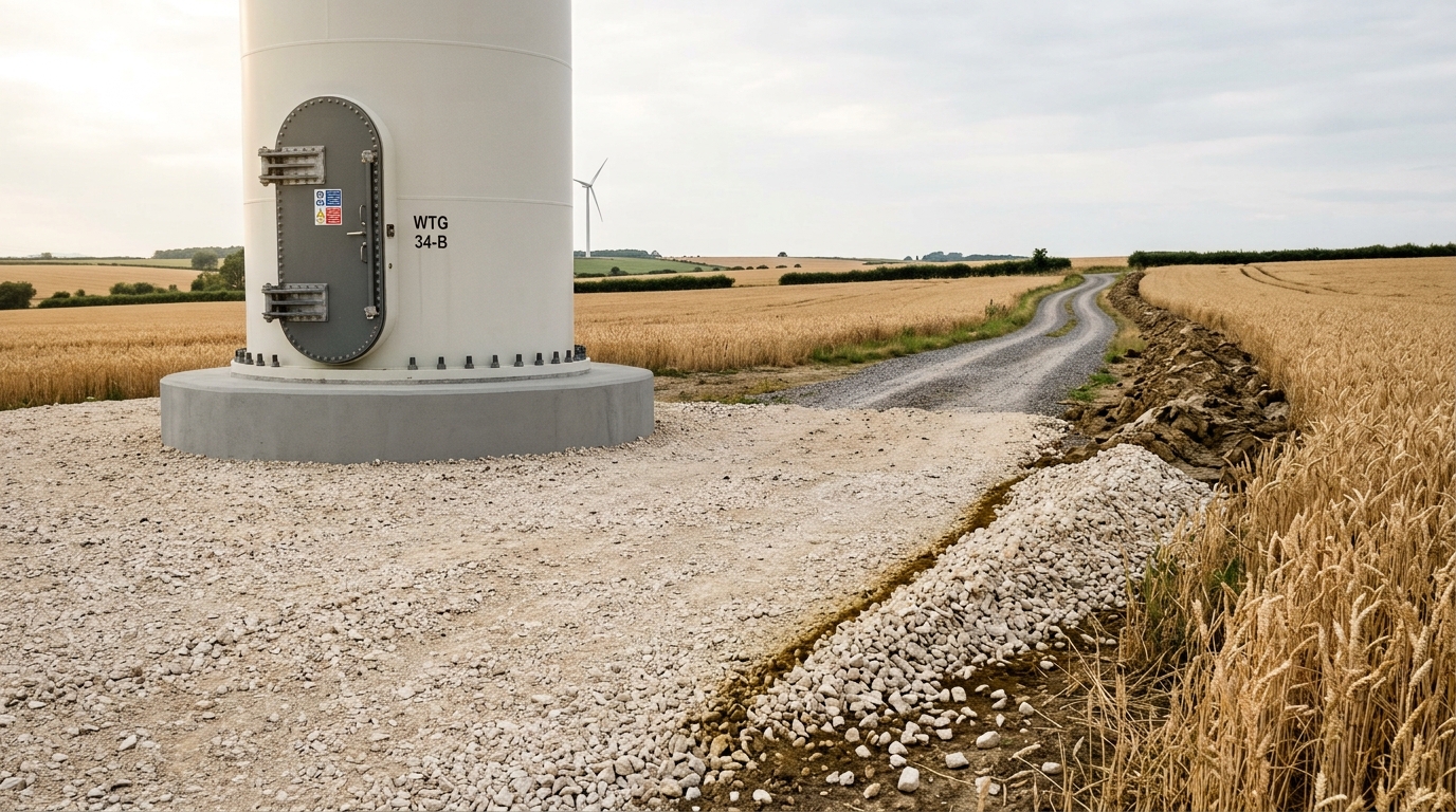
The honest summary is that onshore wind’s power density is somewhere between roughly 0.9 and roughly 7 watts per square metre depending on a definitional choice that no measurement can adjudicate, and that anyone quoting a single figure has silently made that choice for you. The gap between wind and coal survives every convention. The gap between wind and solar does not.
What sub-watt supply would not permit
For most of human history every energy source available was in the band that modern studies now assign to biomass — below one watt per square metre, often far below. Wrigley’s account of the pre-industrial “organic economy” turns on this: societies were “dependent on the annual cycle of plant photosynthesis for both heat and mechanical energy”, so the quantity available each year was capped, and that cap constrained growth [11]. The cap was spatial before it was anything else. Photosynthesis converts sunlight at an overall efficiency Smil puts at no better than 1 per cent, which is why even an intensively cultivated fast-growing tree plantation yields harvest power density around 0.6 watts per square metre [1].
The consequence for settlement is arithmetic. If heat, cooking, draught power and industry all come from land at well under a watt per square metre, then the territory that supports a settlement is enormously larger than the settlement, most people must work that territory, and the size of any town is limited by how far fuel and food can be hauled before the hauling consumes the payload. Smil’s framing of the modern situation inverts this: fossil civilisation secured its most flexible energy carrier by “shifting downward”, generating electricity at one to three orders of magnitude higher density than the densities at which it is consumed in buildings, factories and cities [1]. Pre-fossil societies had no downward shift available. They generated at roughly the density at which they consumed, and their cities were correspondingly rare and small.
Metallurgy is where the constraint bit hardest, because smelting concentrates enormous heat in one place. Straka’s reconstruction of American charcoal iron production gives the parameters: “each ton of pig iron required 180 bushels of charcoal in the furnace”, “600 acres of woodland was harvested annually to fuel the furnace”, and with an average yield of 20 cords to the acre on a 20-year rotation, sustaining one furnace in perpetuity required about 12,000 acres of woodland [12]. Twelve thousand acres is roughly 49 square kilometres held permanently in cycle to keep a single furnace running. The rotation arithmetic reduces to about one cord per acre per year — an annual flow so thin that no amount of organisation could concentrate it further.
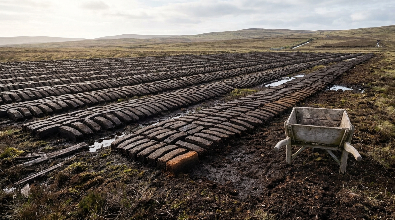
Peat states the same limit more starkly, because peat looks like a fuel stock and behaves like one, but the flow that made it is glacially slow. The World Energy Council gives the organic component of peat a “fairly constant anhydrous, ash-free calorific value of 20-22 MJ/kg”, notes that raw peat is around 90 per cent water and air-dried peat still 40 to 50 per cent, and reports that global mire sequestration of roughly 100 million tonnes of carbon a year exceeds the world’s annual peat harvest by a factor of three to six — a balance that “is not necessarily so on a country or regional basis” [13]. Alexandrov and colleagues put the long-term rate of carbon accumulation associated with peat growth at 18 to 28 grams of carbon per square metre per year [14].
Those two figures permit a rough calculation, and it is worth doing explicitly because the assumption is the interesting part. Take the midpoint of 23 grams of carbon per square metre per year; assume organic matter is about half carbon by mass, giving roughly 46 grams of dry organic matter; apply 21 megajoules per kilogram. The result is close to one megajoule per square metre per year, or about 0.03 watts per square metre. The carbon-fraction assumption is mine and could be off by twenty per cent either way, which does not matter at this resolution. Peat’s renewal rate is one to two orders of magnitude below even a wood plantation. A peat bank is therefore not a low-density renewable flow at all. It is a small, local, slowly recharging stock, and cutting it is mining. The cut trench filling with water is the deposit being spent.
Coal was a density change before it was a quantity change
The usual story is that coal supplied more energy. It did, but the transformative part was that it supplied energy from far less ground. Wrigley’s point is that the energy source remained plant photosynthesis; what changed was that it had been “accumulated over a geological age” rather than harvested annually [11]. A stock accumulated over geological time and extracted through a shaft has a power density that has nothing to do with the flux of sunlight on the surface above it. Smil’s figures for the whole coal system — mining, storage, environmental controls, settling ponds and generation together — range from about 100 to 1,000 watts per square metre, and for the plant alone commonly exceed 2,000 [1].
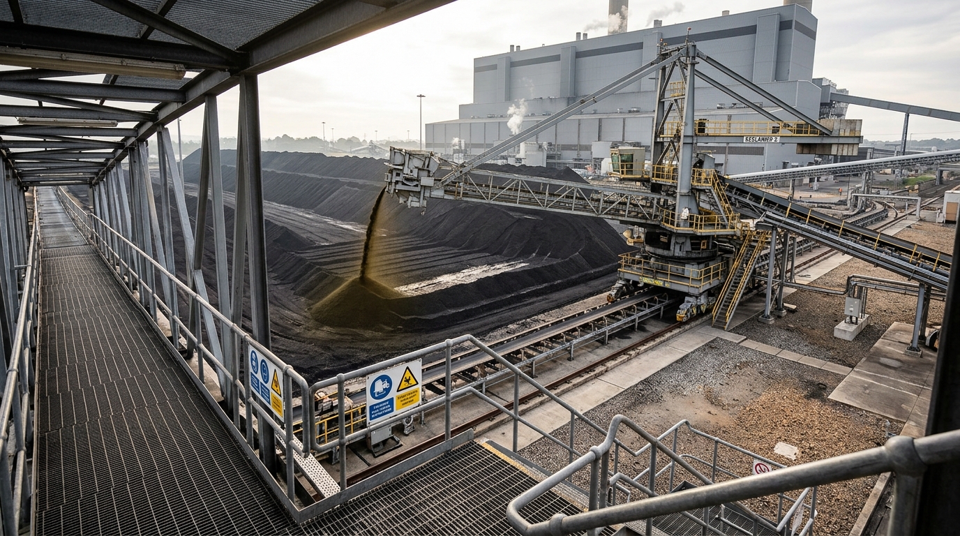
That is what the coke-smelting transition really bought. It did not merely give ironmasters more fuel; it detached the furnace from the 12,000 acres. Once a furnace’s fuel came from a shaft rather than a rotation, output could scale without the woodland scaling with it, and works could sit where ore, water and transport were rather than where forest was. The same release explains dense industrial cities, year-round manufacturing, and the collapse of the share of the population that had to work the land.
It is worth stating what this argument does not establish. High power density did not cause industrialisation; institutions, capital markets, wage structures and prior technical knowledge all sit in that causal chain, and economic historians disagree sharply about their weights. Power density describes a constraint that was lifted, not a mechanism that pushed.
The reverse transition, and the land it wants
Running the transition backwards means rebuilding supply at densities one to three orders of magnitude lower, and the land shows up in the accounts. NREL’s empirical survey of US solar plants — covering 72 per cent of capacity installed or under construction at the time — found a generation-weighted average total-area requirement of 3.5 acres per gigawatt-hour per year, with direct-impact area at 2.9, and capacity-weighted figures of 8.9 and 7.3 acres per megawatt [15]. Converting the total-area figure gives roughly 8 watts per square metre, which sits between Miller and Keith’s measured 5.4 and Nøland’s 9.91 and above Smil’s 4-to-9 bracket.
Van Zalk and Behrens applied their medians to NREL scenarios and found the electricity sector’s footprint growing in every mainland state under an 80 per cent renewable pathway, with Vermont and Washington exceeding 20 per cent of available surface area by 2050 — a result they attribute partly to wide hydropower uncertainty and to modelling that allocates generation by state without accounting for land competition [3]. Smil’s more famous version, as summarised by Vettese, is that a solar-wind-biofuel regime would need the whole land area of the United Kingdom or Germany, and between a quarter and a half of United States territory [10]. Those are conclusions built on assumed densities and assumed demand, and both assumptions are contestable.
The counterarguments, stated properly
Dual use. Most of the area inside a wind farm boundary is not occupied by anything. Smil concedes this himself: “Most of the area occupied by large wind farms could be used for crops or grazing”, while adding that other uses are excluded, access roads must be built and maintained, and buffer zones unsuitable for permanent habitation are created [1]. Van Zalk and Behrens make the same qualification, noting that “increased land-use does not always imply increased competition with other sectors” [3]. For solar, dual use is no longer hypothetical. Barron-Gafford and colleagues, running an agrivoltaic installation in the Sonoran Desert, measured daytime air temperatures 1.2 ± 0.3 degrees Celsius lower under panels, chiltepin pepper fruit production three times greater, cherry tomato production twice as great with 65 per cent greater water-use efficiency, and jalapeño yields essentially unchanged but achieved with 65 per cent less transpirational water loss [16]. That is a genuine result on three crops at one site in one climate, and it should not be extrapolated to cereals in temperate latitudes without evidence.
Offshore siting. Offshore wind moves the denominator off land entirely. Nøland and colleagues put offshore wind’s mean spatial density at 3.89 watts per square metre against 2.12 for onshore [8]; Enevoldsen and Jacobson report European offshore at 2.94 output watts per square metre with a mean capacity factor of 40.8 per cent — lower density than their onshore figure but markedly better utilisation [7]. Sea surface is not free of competing claims, but it is not farmland.
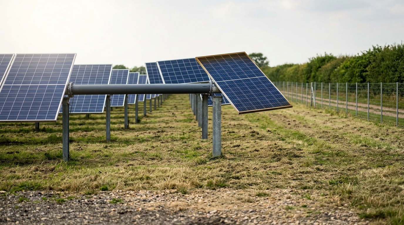
Rooftops. Jacobson’s estimate for rooftop and canopy photovoltaics, at 30 to 40 watts per square metre of panel with conservative capacity factors, is roughly six to eight times the figure Miller and Keith reported for the ground-mounted fleet [6]. Even van Zalk and Behrens, working from the published literature rather than advocacy, found residential photovoltaic mean densities of 6.7 watts per square metre against 5.8 for utility-scale, since rooftops are already tilted and need no service spacing [3]. Rooftop area is genuinely additional to the land budget.
Land is often not the binding constraint. This is the strongest objection, and it is empirical. Lopez and colleagues catalogued more than 1,800 local wind ordinances and more than 800 solar ordinances in the United States in 2022 and found that extrapolating those setbacks nationally could reduce wind and solar resource by up to 87 and 38 per cent respectively [17]. Where a setback rule removes six times more developable area than the panels themselves would occupy, the physics of watts per square metre is not what is limiting deployment. Transmission queues, capital cost, supply chains, grid flexibility and local consent frequently bind first.
Why the metric is partial
Vettese’s review, which grants that the concept is “a useful contribution”, also states the limitation plainly: Smil “does not countenance eco-austerity”, nor does he “question how broader social and economic structures reproduce such wasteful and prodigious expenditures of energy” [10]. Power density takes demand as given. It answers how much ground a given quantity of energy requires, and is silent on whether that quantity is necessary. A halving of consumption halves the land requirement without changing a single density figure.
Four further limits follow from what the metric is:
It is a ratio, so it hides distribution. Nøland’s hydropower mean of 33.73 with a standard deviation of 157.28 is a warning that averaging over incommensurable sites can produce a number with no referent [8]. It is silent on everything but area — emissions, materials intensity, water, waste, cost and dispatchability all sit outside it, and no ranking of technologies should be built from it alone. Its denominator is a convention, as the wind literature demonstrates at length [9]. And it treats all land as fungible, which is exactly what land is not: a hectare of desert, a hectare of intact peatland and a hectare of arable are not interchangeable, and peatland in particular is a carbon store whose disturbance carries a cost the metric cannot see [14].
Even the comparisons that look most robust rest on judgement calls. Van Zalk and Behrens explain part of their divergence from Smil by capacity factor assumptions: Smil applied 70 per cent to biomass against the 32 per cent US national average they used, and 70 to 80 per cent for coal against their 53 per cent [3]. Those are defensible choices from different periods, not errors, and they move the results substantially.
What it is good for, and a testable expectation
Power density is best understood as a constraint detector, not a decision procedure. It identifies where a plan implies a spatial commitment that its authors have not costed, and it explains historical possibility better than almost any other single number: why charcoal metallurgy stalled, why pre-fossil cities stayed small, why a peat bank heats a house and not a foundry.
A prediction, with its conditions attached. Horizon: the next decade, to 2036. Assumptions: continued growth in utility-scale wind and solar in the United States and Europe, no discontinuous change in module efficiency, and no national pre-emption of local siting authority. Claim: disputes about renewable siting will continue to be settled by ordinance, transmission access and consent rather than by land scarcity, and the peer-reviewed range for onshore wind power density will remain wide — spanning at least a factor of three — because the underlying disagreement is definitional. Observable indicators: further multi-method papers of the Covey type reporting method-dependent spreads rather than convergence; continued growth in setback ordinances; land-constrained rejections remaining rare relative to consent-constrained ones. Disconfirmation: if a standards body or a widely adopted protocol fixes a single boundary definition for wind plant area and subsequent studies cluster within, say, twenty per cent, the definitional claim is wrong and power density will have become a measurement rather than a convention. Equally, if deployment in a major market stalls with siting approvals available and land identified as the limiting factor in project-level post-mortems, the constraint hierarchy proposed here fails.
The peat ground remains the useful image. It shows an area being spent, a stock being mined, an unfinished row of turves that will heat one house for one winter. Power density is the number that lets that ground be compared with a gas turbine on a concrete pad, and that comparison is worth having. It is not the number that decides which one we should build.