
Ask an economic historian how fast steam power actually spread through British industry, or how much better off a mill worker’s family was in 1840 than in 1780, and the honest answer starts with a caveat: nobody in that era was collecting the statistics we would want. There was no national income accounts office, no patent-classification database, no firm-level productivity survey. Every quantitative claim about an industrial revolution or a general-purpose technology is therefore a reconstruction — built from records that were kept for entirely different reasons (probate, taxation, patent registration, mill inspection) and repurposed, with known and stated error, into economic statistics. This is a practitioner’s account of three of the core methods behind that reconstruction: rebuilding historical income and wage series from incomplete archives, using patent records to measure how a technology actually diffused, and running firm-level productivity studies from surviving business ledgers. Each method is anchored to a specific published study so the claims here can be checked against their sources rather than taken on faith.
What a “general-purpose technology” claim is actually asserting
Before the method, the term. Timothy Bresnahan and Manuel Trajtenberg introduced “general-purpose technologies” (GPTs) to formalize why a small number of technologies — the steam engine, the electric motor, the semiconductor — seem to drive growth across an entire economy rather than a single sector [1]. Their definition has three specific, testable components: pervasiveness (used across many sectors), inherent potential for continued technical improvement, and “innovational complementarities” — the property that a GPT’s productivity payoff rises as downstream sectors invent their own applications and organizational changes around it, which is why adoption is slow and payoffs lag invention by decades. This is an analytical framework, not a raw statistic; when this article calls something a GPT claim, that is the specific mechanism being asserted, not just a loose way of saying “important technology.”
The empirical implication that matters most for what follows is the lag. Nicholas Crafts applied growth accounting — decomposing measured output growth into contributions from capital, labor, and a residual — to nineteenth-century British steam power and found that steam contributed almost nothing measurable to growth before 1830, and only reached its peak contribution around 1850, roughly a century after Newcomen’s and Watt’s engines were commercially available, once high-pressure steam made the technology cheap and light enough for widespread factory and locomotive use [2]. That is a fact about the shape of a diffusion-driven growth contribution, not a vendor claim about steam’s importance in general — the number comes from a specific growth- accounting calculation applied to specific capital-stock and output series, and it is worth remembering when reading any claim that a new technology’s economic effects should already be visible a decade after invention.
Method one: reconstructing GDP and real wages backward
There was no eighteenth-century national accounts office, so historical GDP and wage series for Britain before the 1850s are built by splicing together output-side estimates (agricultural yields, industrial output proxies, trade records) and price/wage series drawn from an entirely different kind of document: parish records, probate inventories, tax assessments, and institutional wage books. The landmark example is Broadberry, Campbell, Klein, Overton, and van Leeuwen’s reconstruction of British national income back to 1270, which used tithe records, manorial accounts, and urbanization rates as proxies where direct output data does not exist, and cross-validated overlapping proxy series against each other in the years where two or more happen to survive [8]. The core technical move is exactly this cross-validation: no single source covers the whole period at consistent quality, so the practitioner’s job is to find where an earlier, sparser series and a later, denser series overlap, check that they agree in the overlap years within a stated margin, and splice at that point rather than at an arbitrary calendar boundary. Where the two proxy series disagree in an overlap window, that disagreement is itself reported as an uncertainty band on the spliced series, not silently resolved by picking whichever number seems more plausible.

Real-wage reconstruction has its own well-documented controversy that illustrates the same methodological point from a different angle: the same nominal wage records can support very different real-wage conclusions depending on which cost-of-living deflator, and which assumptions about unemployment, household dependents, and urban cost-of-living penalties, are applied to them. Charles Feinstein’s 1998 reassessment recalculated British working-class real earnings from 1770 to 1870 using revised cost-of-living weights and explicit adjustment for the additional living costs of moving to cities, and found that average real earnings rose by less than 15 percent across the 1780s-to-1850s span — far below the more optimistic estimates that had circulated before, and a figure that reopened the long-running “standard of living” debate about whether industrialization’s early decades made ordinary British workers better off [4]. This is worth stating precisely as a methods lesson: the underlying nominal wage data had not changed: what changed the conclusion was the deflator and the adjustment assumptions applied to the same records. Any reader encountering a real-wage claim from this period should ask which price index and which adjustment set produced it, because different defensible choices genuinely produce different answers — this is a case where reasonable experts disagree on method, not one where a single “true” number exists and one side got the arithmetic wrong.
Method two: patent records as a diffusion instrument, and its limits
Patent counts are the most commonly used quantitative proxy for the pace and location of innovation in this period, because patent registries are one of the few near-continuous, dated, and geographically located innovation records that survive from the eighteenth and nineteenth centuries. The classic methodological template for turning a count of individual innovations into a rate of economically meaningful diffusion is not, strictly, a patent study at all: Zvi Griliches’s 1957 study of hybrid corn adoption across US counties modeled the fraction of a region’s farmers adopting the new seed as a logistic (S-shaped) curve over time, and showed that the parameters of that curve — how early adoption started in a county, and how fast it accelerated once started — correlated with the profitability of switching in that county’s local conditions [3]. This logistic-diffusion framework, developed for a twentieth-century agricultural innovation, became the standard tool economic historians later applied to nineteenth-century industrial technologies: count adopting units (firms, counties, patent classes) per period, fit an S-curve, and interpret the curve’s midpoint and steepness as measures of how fast and how completely a technology actually spread, rather than treating the invention date alone as if adoption were instantaneous.

Applying this to patent archives requires classifying each entry by technology and by industry before it can be counted at all, and this classification step is where most of the real archival labor happens and where most of the caveats belong. Petra Moser’s study of patenting at the 1851 Crystal Palace and 1876 Centennial world’s fairs illustrates both the payoff and the limit of this approach directly: rather than relying on official national patent-office counts, which differ sharply across countries with different patent-eligibility rules, Moser built a new dataset of nearly fifteen thousand exhibited innovations — including many never patented at all — classified by industry, and compared countries with and without patent laws. The finding was that patent laws showed no evidence of increasing the overall level of innovative activity, but strong evidence of shifting which industries innovation concentrated in, toward sectors where patenting was easier to enforce [7]. The methodological point generalizes beyond this one study: a raw patent count measures patenting activity, not innovation activity, and the gap between the two varies by country, era, and industry in ways that must be independently established (as Moser did, by building a patent-independent innovation count to compare against) rather than assumed away. Any patent-based diffusion claim in the literature carries this same burden of proof, and a reader should look for whether the underlying study cross-checked patent counts against an independent measure of the activity it claims to track.
Diego Comin and Bart Hobijn’s broader technology-diffusion dataset extends this logistic-curve approach across two centuries and 166 countries and 15 technologies, using output-based adoption measures (installed capacity, units in use) rather than patents where such records survive, and report an average lag of 45 years between a technology’s invention and a country’s adoption of it, with newer technologies diffusing faster than older ones and cross-country diffusion differences statistically accounting for at least a quarter of measured per-capita income differences [6]. That 45-year average is a descriptive statistic averaged across a specific 15-technology, 166-country panel — it is not a universal law of diffusion, and the paper’s own finding that newer technologies diffuse measurably faster than older ones is itself evidence that the average lag is not stable across eras; a scenario in which some future general-purpose technology diffuses on a similarly multi-decade timescale is a plausible extrapolation from this pattern, not a prediction the data can itself confirm.
Method three: firm-level productivity from surviving business records
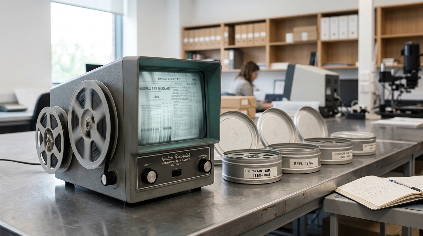
The third method works at a finer grain than national statistics or patent counts: reconstructing productivity at the level of an individual firm, using whatever machinery inventories, output ledgers, and wage books happen to survive in a company’s own archive or a regional record office. This is the method behind the growth-accounting exercises discussed above, at the level a single mill or works, and the archival reality of it is unglamorous and central at once: a firm-level productivity study depends entirely on which specific ledgers survived a given company’s closure, fire, or move, so firm-level samples in this literature are never a random sample of firms — they are a survivorship-biased sample of firms whose paperwork happened to be kept, a limitation every serious study in this tradition states explicitly rather than treating its sample as representative of the whole industry.

The practical steps are consistent across studies of this kind. First, a machinery inventory — often produced for insurance valuation, probate, or an internal stock-take rather than for any economic purpose — is used to estimate the firm’s physical capital stock in a given year: number and type of looms, spindles, or engines, sometimes with a stated horsepower or purchase price that lets the historian convert heterogeneous machines into a comparable capital measure. Second, an output or sales ledger (or, failing that, a raw-material input ledger, used as a proxy for output via a known input-output ratio for the product) supplies the output side. Third, a wage book supplies the labor input, usually more reliably than either of the other two because wage payment was a legal and contractual obligation firms had strong incentive to record accurately even when they had no reason to record capital or output carefully. Total factor productivity is then computed the same way at firm level as Crafts computed it at national level: output growth minus a weighted average of capital and labor growth, with the residual attributed to technological and organizational change. The identification problem specific to this micro-level version is that a single firm’s ledgers rarely supply a long enough continuous run to estimate this residual with much statistical confidence, which is why the credible studies in this tradition build up from many individual firms in the same industry and region rather than resting a general claim on one company’s books, however complete those books happen to be.

Paul David’s classic account of the electrification of American factories supplies the sharpest illustration of why this firm-level, mechanism-level detail matters more than an aggregate growth number on its own. Electric motors were commercially available and individually more efficient than steam engines well before American factory productivity showed any corresponding jump; David’s explanation, built from factory layout records and the archives of firms that undertook electrification, is that the early productivity payoff was blocked by an organizational bottleneck rather than a technical one — factories built around a single central steam engine driving all machinery through overhead line-shafts had to be physically redesigned around distributed, unit-drive electric motors placed at each machine before the efficiency gains of electricity could show up in the output data, and that redesign took decades and a generation of managers willing to abandon their existing factory floor plan [5]. This is the concrete case behind the general GPT claim above about slow, complementary-innovation-driven diffusion: the mechanism was not “electricity was adopted slowly,” but specifically that a distinct, identifiable organizational choice (centralized versus distributed power) determined when the productivity gain became visible, and that mechanism was only established by matching firm-level layout and productivity records against each other, not by reading off an aggregate electrification-adoption curve alone.
Reading a historical-statistics claim as a practitioner would
Bringing these three methods together yields a short discipline for reading any specific claim about industrial-revolution economics rather than accepting it wholesale. First: is the number a direct measurement, or a reconstruction spliced from proxy series, and if the latter, where is the overlap window that was used to validate the splice? Second, if the claim rests on patent or innovation counts, has the study independently checked whether patenting activity actually tracks the underlying innovation it claims to measure, the way Moser’s exhibition-based dataset did, or is it assuming the two move together? Third, if the claim is at firm level, how many firms and what selection process produced the surviving sample, and does the study state that limitation openly? A claim that fails to answer these questions is not necessarily wrong, but it has not yet earned the confidence its narrative framing usually implies.
It is worth being explicit, too, about which of the paragraphs above are fact, which are analysis, and which slide toward scenario. The 1830-to-1850 lag in steam’s growth contribution, the sub-15- percent real-wage rise Feinstein calculated for 1780s-to-1850s Britain, Moser’s null finding on patent laws and innovation levels, and the 45-year average adoption lag in Comin and Hobijn’s panel are each a specific reported statistic from a named, checkable study, not this article’s own estimate. The claim that firm-level TFP studies are inherently survivorship-biased, and that electrification’s delay was organizational rather than technical, are this article’s synthesis of what those studies’ own stated methods and findings imply — a reasonable reading, but an inference rather than a number lifted directly off a page. And any extension of the 45-year diffusion-lag pattern to a future general-purpose technology, artificial intelligence included, is a scenario: it assumes that whatever organizational-complementarity bottleneck slowed nineteenth-century electrification (a real, firm-level, physical-relayout cost) has a genuine present-day analogue, and it would be disconfirmed by observing rapid, complementary-innovation-free productivity gains following that technology’s release, the way David’s data show did not happen with electricity but in principle could happen with a technology that requires no comparable physical or organizational reconfiguration to use.
One further practical point deserves its own space, because it is where a great deal of published disagreement in this literature actually originates: uncertainty in these reconstructions is rarely a single error bar around a single number. It is usually several distinct sources of uncertainty stacked on top of each other, each with a different shape. Sampling uncertainty, from how many parishes, firms, or gazette years happen to survive, behaves roughly the way a statistician expects — it shrinks as more surviving records are added and can be summarized with a confidence interval in the ordinary sense. Classification uncertainty, from how a given patent, ledger entry, or occupation title is assigned to a category, does not shrink with more data at all, because adding more records classified under the same ambiguous scheme just repeats the same judgment call at larger scale; it is instead addressed by re-coding a sample under an alternative scheme and reporting how much the headline number moves, which is exactly what Moser did in building an independent, patent-law-free innovation count to check against raw patent totals [7]. Deflator and index- construction uncertainty, the kind Feinstein’s reassessment turned on, does not shrink with sample size either; it is addressed by publishing the sensitivity of the headline figure to the specific price weights and adjustment assumptions chosen, so a reader can see how much of a “pessimist” versus “optimist” standard-of-living conclusion rides on the deflator alone rather than on the underlying wage records [4]. A practitioner reading a historical-statistics paper learns to ask which of these three kinds of uncertainty dominates a given headline number, because the appropriate response differs: more archival digitization helps the first, an independent cross-check helps the second, and an explicit sensitivity table helps the third, and conflating them is the most common way a popular summary overstates the precision of a historical economic claim.
A related caution applies specifically to any cross-period comparison of a GPT’s growth contribution, of the kind this article has made between steam, electrification, and by extension any future general-purpose technology. Crafts’s steam growth-accounting exercise and David’s account of electrification’s organizational lag were each built from that technology’s own specific capital- stock, wage, and factory-layout records, assembled under that era’s own available archives [2, 5]. Placing their findings side by side to argue that GPTs generally take multiple decades to show up in aggregate productivity, as Bresnahan and Trajtenberg’s framework predicts they should, is a defensible analytical synthesis, because the underlying mechanism (complementary reorganization has to precede the productivity payoff) is stated in both studies independently rather than assumed by the comparison itself [1]. But it stops being a fact about GPTs in general the moment a third, structurally different technology is folded into the same claim without its own equivalent archival study behind it. The discipline that holds for a single case holds just as strictly across cases: a comparative claim is only as strong as the weakest of the individual studies feeding it, and stating which specific study supports which specific piece of a multi-technology argument is not pedantry, it is the difference between a supported comparison and a plausible-sounding one.
None of this is a case for skepticism about historical economics as a field; it is a case for reading its numbers the way its own best practitioners produce them; as reconstructions built from specific, imperfect, repurposed archives, with the splice points, classification choices, and sample limits stated alongside the headline figure, rather than as facts that arrived already measured.