Why Materials Fail: Fracture, Flaws and the Inspection Interval

The strength you calculate is not the strength you measure

Take the bond energy of a crystalline solid, estimate the stress required to pull two atomic planes apart against it, and you arrive at a theoretical cohesive strength on the order of a tenth of the elastic modulus. Then test the material. Ordinary glass, ordinary steel and ordinary ceramic all fail at a small fraction of that figure, and the discrepancy is not a rounding error or an artefact of impure specimens. It is one to three orders of magnitude, and it is completely reproducible.

For most of the nineteenth century this was simply the way of things: engineers measured strength, tabulated it, and applied a factor of safety large enough to absorb their ignorance. The factor of safety was, in effect, a numerical confession. It encoded the observation that structures fail in ways that a strength number does not predict, without saying anything about why.

A. A. Griffith’s 1921 paper is the moment the confession becomes a theory ^[1]. Griffith’s move was to stop treating the solid as a continuum that happens to break, and to treat it as a body that already contains cracks. As John Knott put it in a centenary commentary for the Royal Society, Griffith “invoked the concept of inherent flaws in the material: what came to be referred to as Griffith cracks”, and then produced an analysis of fracture strength based on the balance between released elastic strain energy and the energy required to create two new free surfaces ^[2].

That reframing is the whole of what follows. Failure is not the material running out of strength. It is a pre-existing defect finding conditions under which it pays, energetically, to grow.

A crack is a lever for stress

The first half of the argument is purely elastic and predates Griffith. An elliptical hole in a stressed plate does not merely remove load-bearing material; it redistributes the stress that would have passed through that material into the region around the hole’s sharpest curvature. For an elliptical flaw of half-length $a$ and tip radius of curvature $\rho$ in a plate under remote tension $\sigma_\infty$, the peak stress at the tip is approximately

Three things follow. First, the concentration depends on the flaw’s aspect ratio, not on its absolute size — a long shallow scratch and a short sharp one can concentrate stress equally. Second, as the tip sharpens toward an atomically sharp crack, $\rho \to 0$ and the predicted peak stress diverges. Third, and most usefully, a designer cannot avoid stress concentration by making the part thicker; the concentration factor is geometric.

The divergence is where the elastic argument stops being sufficient. If stress at a sharp crack tip is unbounded, every cracked body should fail under any load at all, and they visibly do not. Something must limit either the stress or the relevance of the stress. The resolution is that stress at a mathematical singularity is not the right criterion for fracture, because no real material sustains it — the tip blunts, yields, or bonds simply break over a finite process zone. What survives the singularity is not a stress value but the rate at which energy is released as the crack lengthens.

Griffith’s exchange rate

Griffith’s criterion is an accounting statement. Extending a crack by a small increment releases stored elastic strain energy from the material that unloads around the new crack faces, and consumes energy in creating those faces. If the release exceeds the cost, extension is spontaneous and the crack runs. For a through-thickness crack of half-length $a$ in a linear-elastic plate with modulus $E$ and surface energy $\gamma_s$, the critical remote stress is

The structure of this expression matters more than its coefficients. Strength scales as the inverse square root of flaw size, so halving the largest flaw raises strength by roughly forty per cent, and doubling it costs about thirty per cent. Strength is not an intrinsic property at all in this picture; it is a joint property of the material and its worst defect. Griffith’s own experimental work was on glass, where the assumption of negligible plastic deformation is nearly exact and the theory therefore lands cleanly ^{[1, 2]}.

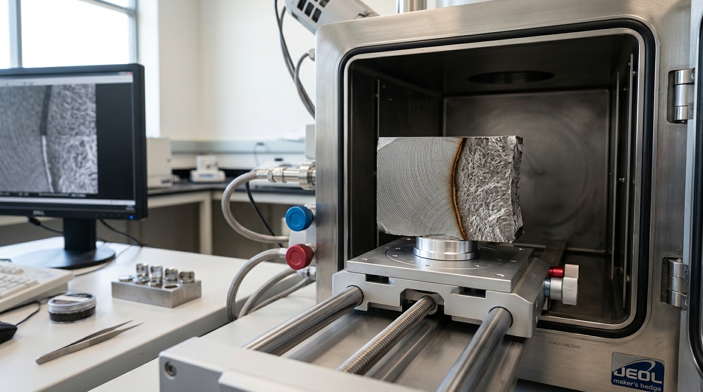
Applied directly to metals, the criterion underpredicts fracture stress badly, because $\gamma_s$ accounts only for the two new surfaces. In a metal, the overwhelming majority of the energy consumed goes into plastic work in a zone ahead of the tip — dislocation motion, void nucleation, blunting. The repair is to replace the surface energy with an effective work-of-fracture term that absorbs plastic dissipation. That substitution is conceptually cheap and physically enormous: it can raise the energy cost of crack extension by three or four orders of magnitude, and it is the reason a ductile alloy tolerates flaws that would destroy a glass of the same nominal strength.

Toughness is the design property; strength is a symptom

The modern formalism replaces the energy balance with a field parameter. Near the tip of a crack, the elastic stress field has a characteristic inverse-square-root singularity whose amplitude is set by a single quantity, the stress intensity factor:

Here $\sigma$ is the applied stress, $a$ the crack size, and $Y$ a dimensionless factor capturing geometry and loading. The claim embedded in this expression is a similitude claim: two cracked bodies of different shape and size, loaded differently, have the same crack-tip conditions if they have the same $K$. Fracture then occurs when $K$ reaches a material-specific critical value, the plane-strain fracture toughness $K_{\mathrm{Ic}}$.

This is the pivot from strength to toughness, and it changes what a design calculation is. With a strength allowable, you compute a stress and compare it to a number. With a toughness allowable, you must additionally state a crack size — and the moment you must state a crack size, you have implicitly committed to knowing what flaws your manufacturing process leaves behind and what your inspection can find. A high-strength alloy with low toughness will tolerate a smaller crack than a lower-strength alloy with high toughness, at the same applied stress. Selecting on strength alone systematically selects toward brittleness, because in most alloy systems the two properties trade against each other.

Two caveats belong here rather than in a footnote. The linear-elastic parameter $K$ is only meaningful under small-scale yielding, where the plastic zone at the tip is small relative to the crack and the remaining ligament. When it is not — thin sections, tough alloys, high temperatures — elastic-plastic parameters such as the J-integral or crack-tip opening displacement are required instead. And $K_{\mathrm{Ic}}$ is measured under a standardised constraint condition; a thin plate of the same alloy will exhibit a higher apparent toughness because plane-stress conditions permit more plastic work. Toughness quoted without its measurement conditions is close to meaningless.

Ductile and brittle are conditions, not identities

The most consequential misreading in materials engineering is that ductility is a fixed attribute of a material. It is not. In body-centred-cubic metals — most structural steels among them — the same alloy deforms plastically above a transition temperature and cleaves below it, with the transition sharp enough to be crossed by an ordinary seasonal change in water temperature.

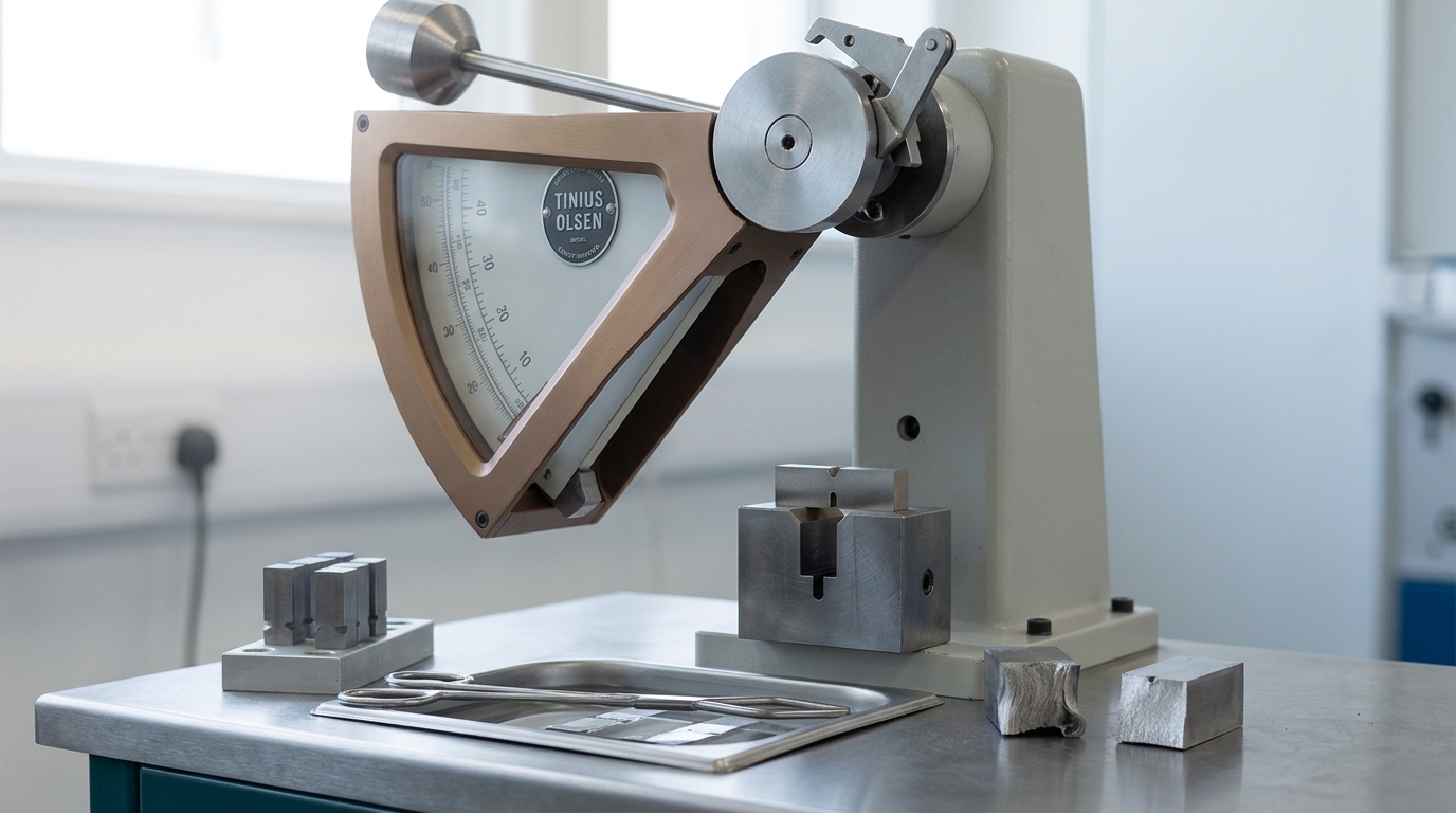
The best-documented illustration is also the one most often told badly. In 1998, NIST published a metallurgical study of steel and rivets recovered from the wreck of the RMS Titanic ^[3]. Using a 27 J criterion, the study reports a ductile-to-brittle transition temperature of approximately plus 40 degrees Celsius for specimens cut in the longitudinal rolling direction and plus 70 degrees Celsius in the transverse direction, against approximately minus 15 degrees Celsius for a modern ASTM A36 mild steel measured the same way. Seawater at the time of the collision was about minus 2 degrees Celsius. The hull steel was, on that measure, deep in its brittle regime.

What the report then does is more instructive than the numbers. It explicitly refuses the popular conclusion that the builders used substandard steel. Sulphur content was above the 1906 standard, but the report traces that standard through revisions to 0.055 per cent in 1933 and 0.05 per cent in 1946 and finds “no evidence that the concentration level was set in reaction to any data linking sulphur concentrations to fracture or tensile behaviour”. It notes that the quantitative link between tramp-element chemistry and brittle fracture was not established until the analysis of Liberty ship failures during and after the Second World War, that the Charpy V-notch test had been devised only about five years before the ship was built, and that in 1911 routine fracture toughness testing was confined to ordnance steels. Its conclusion is that any assertion the builders should have connected a chemical analysis to a fracture risk “is unfounded” ^[3]. This is what careful attribution looks like: the material was brittle at service temperature, and the people who specified it had no framework in which that was a question they could have asked.

The Liberty ship programme is the case that produced the framework. A failure-case database maintained by Japanese failure-analysis researchers records 2,708 Liberty ships built between 1939 and 1945, and 1,031 brittle-fracture damage reports attributed to Liberty ships by 1 April 1946 out of 1,441 cases across 970 cargo vessels — while stating plainly that “these numbers vary by source” and citing an alternative tabulation of 1,289 damaged Liberty ships with 233 sunk or seriously damaged ^[4]. The same entry is internally inconsistent about whether one frequently pictured vessel that broke in two at its outfitting berth was a Liberty ship or a T-2 tanker. Both facts are worth stating: the aggregate pattern is solid and the individual anecdotes are not, which is precisely why the programme’s lesson had to be extracted statistically rather than from a single dramatic photograph.

The mechanism the investigation converged on combines three conditions that raise the transition temperature or the local stress state: low temperature, high loading rate, and triaxial constraint from section thickness or a structural notch. Welded construction removed the crack arrest that riveted seams had incidentally provided, so a crack initiated at a weld defect or a hatch corner could traverse a hull rather than stopping at a plate boundary. The programme’s cost bought the discipline: the case record explicitly identifies the recognition of these problems as the start of fracture mechanics as an engineering discipline ^[4].

Fatigue is the failure mode that actually dominates service

Everything so far concerns a single application of load. Most components in service never see a load approaching their static limit and fail anyway, because cyclic loading accumulates damage at stresses far below yield. Fatigue is not a weaker version of overload; it is a different process, in which a crack initiates at a stress raiser, grows a small increment per cycle, and finally reaches a size at which the remaining ligament fails in a single event that looks like overload but is not.

The governing correlation is empirical. Paris and Erdogan proposed that crack growth per cycle depends on the range of the stress intensity factor over the cycle:

The parameters $C$ and $m$ are fitted, not derived, and depend on environment, frequency, temperature and stress ratio. A mechanics review that proposes a generalised form of the law opens by conceding that “fatigue life prediction is still very much an empirical art rather than a science”, and notes that the power law holds only in an intermediate regime, deviating near the threshold below which cracks do not propagate and again in the fast-growth stage approaching final fracture ^[6]. The same review sets out the live disagreement in the field: short cracks, comparable in size to the microstructure or to the local plastic zone, grow at rates that the long-crack law does not describe, and there is no consensus on whether a single stress-intensity-based similitude parameter can be repaired to cover them or whether short-crack behaviour requires a separate model with its own length scale ^[6]. Practitioners who need a number today generally handle this by treating the threshold conservatively rather than by resolving the physics.

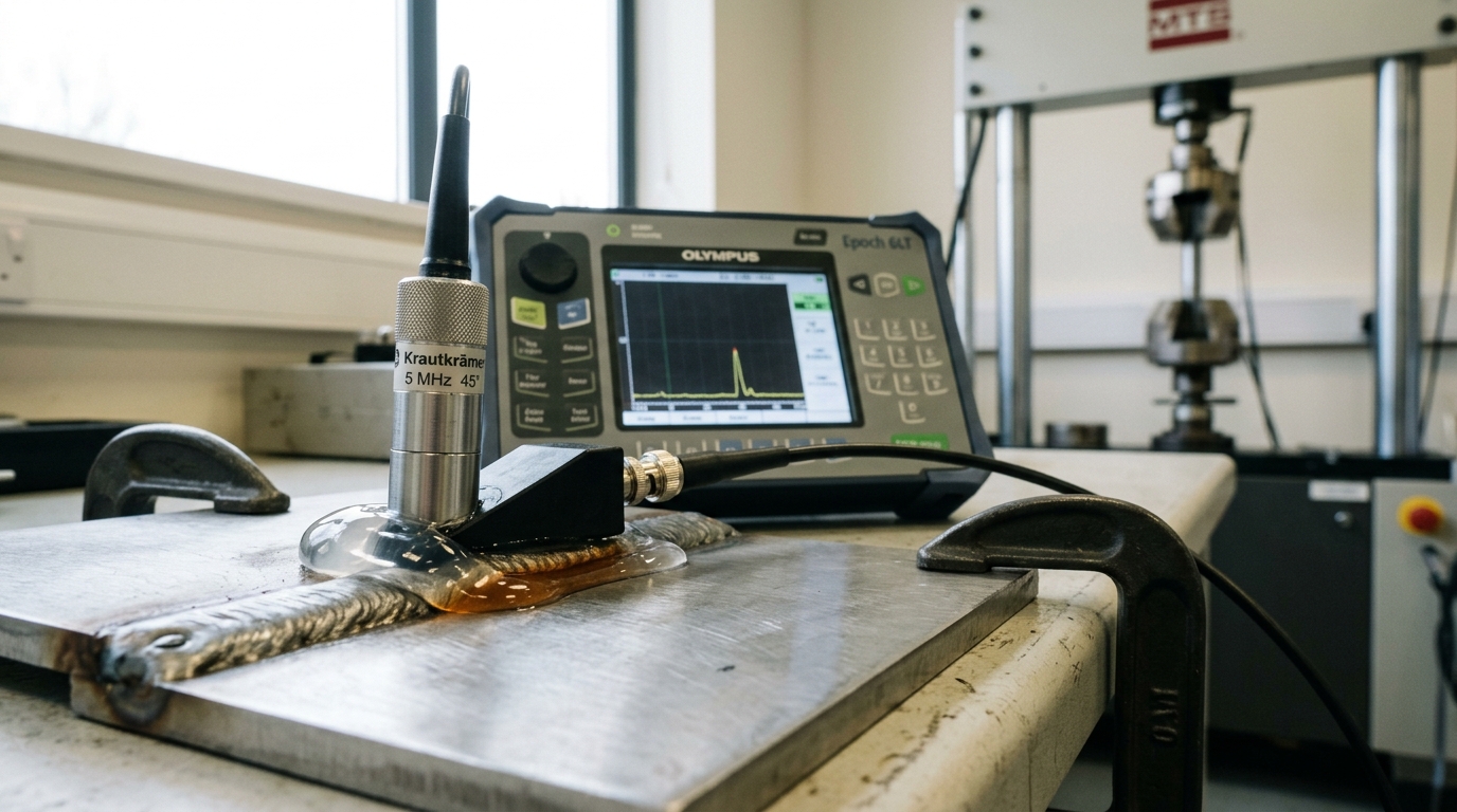
Two aviation cases anchor what this costs when it is ignored, and both have been re-analysed with tools their investigators did not have. The de Havilland Comet I losses of 1954 were traced by the Royal Aircraft Establishment to structural failure of the pressure cabin brought about by fatigue. Withey’s later reanalysis applied fracture-mechanics methods that were not available in 1954 and estimated the initial defect size in G-ALYP at approximately 100 micrometres — a size, he notes, “not incompatible with the manufacturing techniques of the time” ^[5]. A hundred-micrometre defect is invisible to the inspection regime of the period and irrelevant to any strength calculation. It was nonetheless sufficient, under repeated pressurisation cycles at a cabin cut-out, to end the programme.

Thirty-four years later, an Aloha Airlines Boeing 737 lost roughly five and a half metres of upper fuselage skin in flight near Maui. The NTSB investigation raised, as a central safety issue, multiple-site fatigue cracking of the fuselage lap joints — many small cracks growing independently at adjacent fastener holes, each individually below the size an inspector would act on, which link up to form a crack far longer than any single one ^[7]. Multiple-site damage is the specific failure mode that breaks the reassuring arithmetic of damage tolerance, because the residual strength of a structure containing twenty short cracks is not the residual strength of a structure containing one short crack.

Creep makes time itself a load variable

At temperatures above roughly forty per cent of the absolute melting temperature, a metal under constant stress deforms continuously. Creep proceeds by dislocation processes at higher stresses and by diffusional transport of vacancies through the lattice or along grain boundaries at lower ones, and it ends in rupture. For turbine blades, boiler headers and pressure vessels, the design life is measured in tens of thousands of hours, which creates an evidential problem with no clean solution.

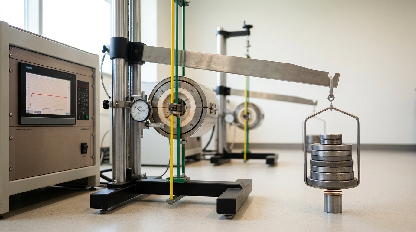
A critical review of creep lifing methods states the difficulty directly: since plant is expected to operate well beyond 100,000 hours, “it is not feasible to conduct 100,000 h creep tests on new materials in order to establish safe operating stresses” ^[10]. Practice is therefore to test at elevated temperature for a few thousand hours and extrapolate using a time-temperature parameter, most commonly the Larson-Miller parameter, which collapses stress-rupture data onto a single master curve. The review’s finding is that the Larson-Miller constant, treated as a material constant, in fact varies with material and condition, and that traditional parametric methods can give non-conservative predictions of rupture time at higher temperatures ^[10]. This is not a marginal statistical caveat. A non-conservative extrapolation in creep means the component reaches its rupture condition earlier than the design calculation says.

The disagreement here is methodological and unresolved. The review argues that stress-normalised approaches such as the Wilshire equations and hyperbolic-tangent models perform better because they are sensitive to a change in the dominant deformation mechanism between test and service conditions ^[10]. Whether that advantage survives across alloy classes and out to service durations that nobody has yet observed is, by construction, not something present data can settle.

Stress-corrosion cracking couples chemistry to mechanics

Some failures require an environment as well as a stress, and are not predicted by either discipline alone. Stress-corrosion cracking occurs when a susceptible alloy, a specific chemical environment and a sustained tensile stress coincide; remove any one and the cracking stops. A recent review catalogues the competing mechanisms — film rupture with anodic dissolution and repassivation, hydrogen embrittlement, surface mobility, internal oxidation, and film-induced cleavage — and does not select among them, because different alloy-environment pairs appear to be governed by different ones ^[9].

The engineering signature is what makes it dangerous. Cracking proceeds at stress intensities far below $K_{\mathrm{Ic}}$, above a threshold conventionally denoted $K_{\mathrm{ISCC}}$; the applied stress can be residual rather than service-applied, and therefore invisible in a load analysis; and the crack can be tight, branched and intergranular, which is close to the worst case for detection. The review’s own summary of why prognosis remains hard is that “the intricate interplay among mechanical, chemical, and electrochemical factors hinders the accurate prognosis of material degradation”, compounded by inconsistent test methodologies across the literature ^[9].

The consequences are not hypothetical. In its report on the 1967 collapse of the U.S. 35 highway bridge at Point Pleasant, West Virginia, the National Transportation Safety Board attributed the failure to a cleavage fracture in the lower limb of the eye of a single eyebar, arising from a flaw that reached critical size over the structure’s forty-year life through the joint action of stress corrosion and corrosion fatigue — in a location that could not have been detected by any inspection method then available without disassembling the eyebar joint ^[8]. Forty-six people died. The failure was not of a material property but of an inspection concept: the structure had no non-destructive route to the surface where the damage was accumulating.

Brittle strength is a distribution, not a number

If the strength of a brittle body is set by its largest flaw, and flaw populations are random, then strength is a random variable and reporting a mean is an error of category. The standard treatment is the Weibull weakest-link model, in which the probability that a body of volume $V$ survives a uniform stress $\sigma$ is

with $m$ the Weibull modulus and $\sigma_0$ a scale parameter. A larger $m$ means tighter scatter. A review of Weibull analysis across ceramics reports moduli of roughly 10 or below for many advanced ceramics such as alumina, hydroxyapatite and silicon carbide, below about 7 for the glass-ceramics and zirconias surveyed, and above 40 for one magnesium-based glass, while emphasising that reliable modulus estimates need substantial sample sizes ^[11].

The practically important consequence is size scaling. Because a larger stressed volume samples more of the flaw population, mean strength falls as the specimen grows, and the ratio of strengths of two specimen geometries goes as the ratio of their effective volumes raised to the power $1/m$ ^[12]. Small-coupon test data therefore systematically overstate the strength of a full-size component, and the overstatement is worse for materials with low Weibull modulus — that is, for exactly the materials whose scatter already makes them hard to design with.

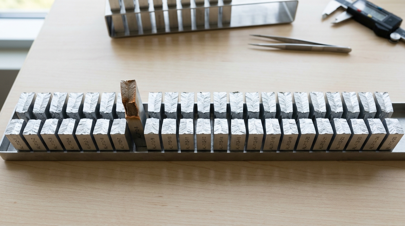
The practice guidance is unusually blunt about sample size. A systematic review of Weibull statistics in materials testing states that estimates of characteristic strength converge quickly as sample size reaches ten or more, but that modulus estimates are highly variable for small sets, so “it is common to require no fewer than ten test specimens and preferably 30 to obtain good estimates of the Weibull modulus”, with bias in the modulus of 5 per cent or more for sets smaller than ten ^[12]. Published strength comparisons based on five specimens per condition are common and, on this analysis, close to uninformative about the parameter that governs reliability. The weakest-link assumption itself also has limits: it presumes a single unimodal flaw population, and a material with both surface machining damage and internal porosity will not follow one straight line on a Weibull plot ^{[12, 11]}.

Failure became an inspection interval

The cumulative effect of everything above is an institutional change, not merely a technical one. If a component fails when a growing crack reaches a critical size, and if crack growth per cycle is a calculable function of load history, then the safety of the component is determined by three quantities: the largest crack that could plausibly be present and undetected, the growth rate under the service spectrum, and the crack size at which residual strength falls to the required level. The distance between the first and the third, divided by the second, is a time. Inspect more often than that time, with a method that reliably finds the assumed initial size, and the structure is safe by construction rather than by optimism.

This logic is written directly into regulation. United States transport-category airworthiness rules require an evaluation showing that catastrophic failure from fatigue, corrosion, manufacturing defects or accidental damage will be avoided across the operational life, and state that “based on the evaluations required by this section, inspections or other procedures must be established, as necessary, to prevent catastrophic failure” ^[13]. The damage-tolerance paragraph ties the assumed extent of damage to detectability and growth: the damage considered for residual strength “must be consistent with the initial detectability and subsequent growth under repeated loads”. After the multiple-site damage experience, the same rule requires a limit of validity — a stated number of flight cycles or hours within which widespread fatigue damage is demonstrated not to occur ^[13].

Spaceflight practice encodes the same idea with different arithmetic, because there is no inspection opportunity in service. NASA’s fracture control standard defines damage tolerance as the concept under which an undetected flaw will not grow to failure during the service life factor times the service life, and requires fracture-critical metallic parts to demonstrate a minimum service life factor of 4, with a factor of 1.5 on alternating stress, using an assumed initial flaw tied to the demonstrated capability of the non-destructive evaluation applied ^[14]. The assumed flaw is not a guess about what is there; it is a statement about what could have been missed.

Two cautions on how this framework is used. First, an assumed initial flaw size is only as good as the probability-of-detection data behind it, and claims by inspection-equipment suppliers about detectable flaw size should be read as vendor assertions until they are supported by independent probability-of-detection trials on representative geometry and surface condition. Second, probability of detection is a property of the whole inspection system — method, access, surface preparation, procedure and inspector — not of the instrument, so a threshold demonstrated in a laboratory coupon programme does not transfer to an in-service joint without evidence.

As a prediction, with a horizon of 2036: continuous structural health monitoring will supplement, but not replace, interval-based inspection for primary structure in regulated transport applications. The assumptions are that certification frameworks continue to require demonstrated residual strength against an assumed flaw, that sensor networks continue to have their own reliability and coverage limits, and that no monitoring modality achieves a validated probability of detection across all critical locations. Observable indicators that this is holding would be monitoring credited as a supplement to, rather than a substitute for, scheduled inspection in approved maintenance programmes. The disconfirming condition is specific: if a civil airworthiness authority approves a primary-structure maintenance programme in which a monitoring system replaces a scheduled damage-tolerance inspection outright, rather than extending its interval, the prediction is wrong.

The deeper point is that fracture mechanics did not make materials safer by making them stronger. It made them safer by changing the question. A strength allowable invites the belief that a part is either adequate or inadequate. A toughness allowable, a growth law and a detectable flaw size together concede that every part contains defects, and ask only whether there is enough time between the smallest flaw that can be found and the largest flaw that can be tolerated. That concession is what turned failure from an unpredictable event into a scheduling problem — and it is why the most consequential number in a modern structural design is often not a stress at all, but a date.