A boosted, spinning wavepacket sits still for no one. An accelerometer, a spin analyzer, a postselected photon count, and a detector array each report a different point for it, and none of the four is wrong by its own rules.
Research paperRevolutionary Life 75, Series D, No. 7 ·
this page is the paper's summary — the full text is the PDF.
Download the paper (PDF)
Four instruments are about to measure the same crossing. Every one of them will be right.
Abstract
A boosted, spinning wavepacket has no single position even after mass, energy, and spin are fixed: five established constructions -- the Newtonian mass centroid, the observer-dependent stress-energy centroid, the commuting-component Newton-Wigner-Pryce operator, a postselected weak-value estimator, and a detector-tied localization POVM -- return different, or differently typed, answers to "where." This article treats that plurality as an atlas. It fixes each chart's auxiliary data, derives the transition function relating a body's centroid as measured by two observers -- a shift bounded by the spin-to-mass length rho_M = |S|/(Mc), saturated at ultrarelativistic boost -- and shows the bound is, by design, ignored by a weak value. It recovers the Newtonian centroid nonrelativistically and the coincidence of the covariant and canonical charts at zero spin, and shows, via Hegerfeldt's and the Reeh-Schlieder theorem, why no sharp chart extends to a fully causal, exactly localized global one. A trapped-ion Dirac simulation and an amplified spin-Hall-of-light measurement anchor two charts in data. This is a synthesis, not a new observable, and no simulation was run to produce it.
ADVERTISEMENT
The Atlas That Refuses to Close
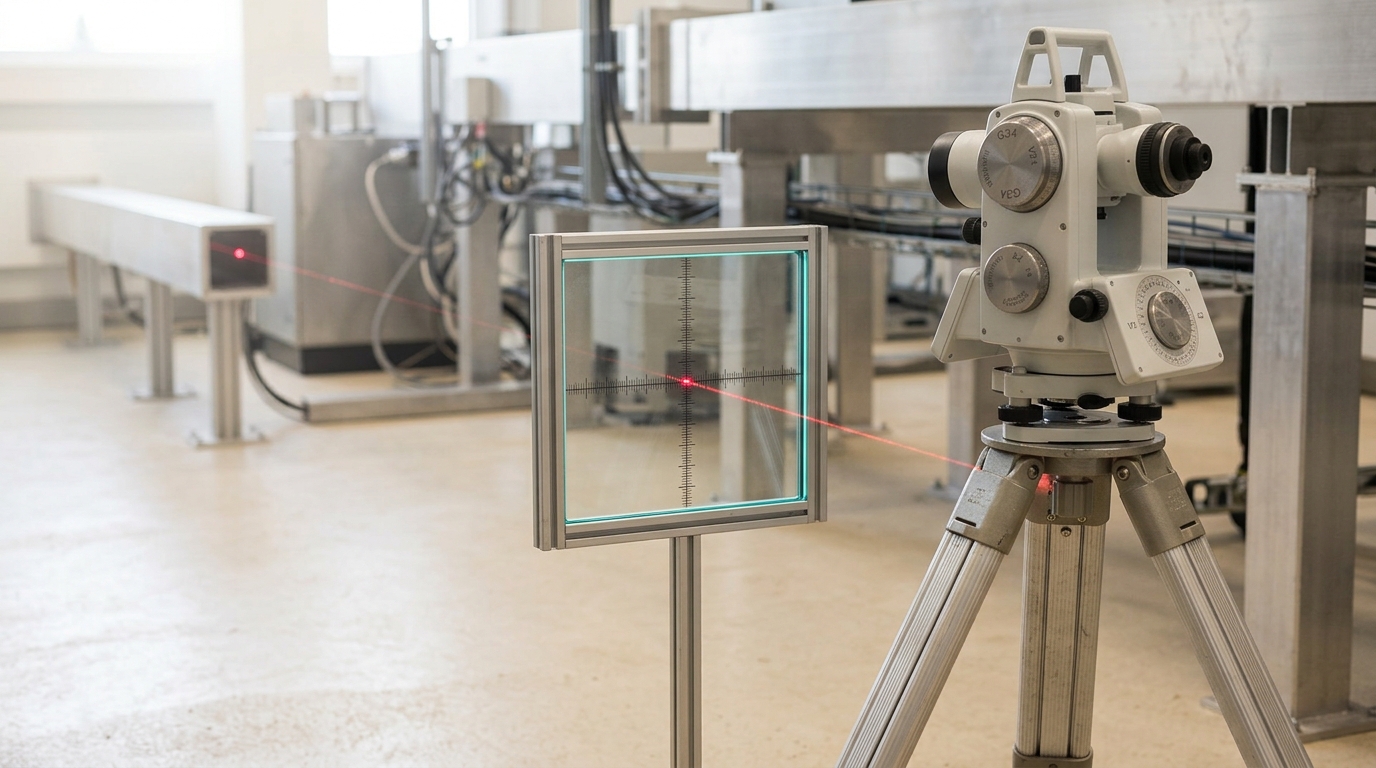
Send a single spin-half particle down a beamline at six-tenths of the speed of light and ask four instruments one question: where is it? An accelerometer riding alongside the beam reports a point fixed by the particle’s own mass distribution in its own rest frame. A spin analyzer downstream reports a different point, shifted transverse to the beam by an amount that grows with the particle’s spin. A weak-measurement stage further along reports a third value, extracted from a postselected sub-ensemble, that need not be a spacetime point at all — it can come back complex. A segmented detector array at the end of the line reports not a point but a smeared probability of where a click occurred, with a width no shrinking of the apparatus can beat below a fixed floor. All four answers are correct. None of them is a mistake, a miscalibration, or a rounding error in someone else’s calculation. They are different, mutually consistent, individually rigorous answers to a question that relativistic quantum mechanics has never let have one answer.
This is not a controversial claim in need of rescue. It has been established, piece by piece, for most of a century: by Pryce’s 1948 classification of every reasonable relativistic centre-of-mass candidate, by Newton and Wigner’s 1949 construction of a position operator with the right commutation relations bought at the price of frame-dependence, by Fleming’s 1965 demonstration of how badly those two properties trade off against each other, and, more corrosively, by Hegerfeldt’s proof that no sharp position operator of any of these kinds can be exactly localized and strictly causal at the same time. What has not existed, across that literature, is a single object that takes the plurality itself as the thing to be measured: a map of which charts exist, what data each one needs to be evaluated, how far apart two charts’ answers can legitimately drift for the same physical state, and where the whole scheme runs out of paper. That is what follows. It borrows no new physics and proposes no new position operator. It proposes only the atlas, and asks the atlas to explain itself.
A Single Instant Is Not a Single Slice
Start with the least controversial position anyone has ever assigned to an extended body: the Newtonian, mass-weighted centroid, RN=∑amara/∑ama↗, a sum over the body’s constituent mass elements ma↗ at positions ra↗, evaluated at one common instant. That last clause is doing all the work relativity is about to object to. “One common instant” means one value of a time coordinate t↗ shared by every term in the sum — the coordinate time of whichever inertial frame is doing the summing, not any single mass element’s own proper time along its own worldline — and which value of t↗ counts as simultaneous with which is exactly the freedom special relativity takes away: two observers in relative motion slice the same set of worldlines into different families of simultaneous events, and a mass-weighted average taken over one observer’s slice need not equal the same average taken over another’s. RN↗ is not wrong. It is incomplete until the slice is named.
ADVERTISEMENT
Naming the slice is the first entry in this atlas’s notation. Let Σ↗ be a spacelike hypersurface and uμ↗ the four-velocity of the observer whose notion of simultaneity Σ↗ represents, with Σ↗ taken orthogonal to u↗. Replace the discrete sum with the body’s stress-energy tensor Tαβ↗ and define the energy centroid
Every quantity here has a declared type. Tαβ↗ is an energy-momentum density, units of energy per volume; dΣβ↗ is a directed three-volume element on Σ↗, units of volume; uα↗ is dimensionless once normalized to uμuμ=−1↗; xμ↗ is a spacetime coordinate, units of length. The factor TαβuαdΣβ↗ appears in numerator and denominator identically and cancels completely, leaving Xμ↗ with units of length — a genuine spacetime point, not a bookkeeping artefact. That is the atlas’s first check, a unit audit passed by construction rather than coincidence, because the same weighting sits on both sides of the ratio.
Xμ(u,Σ)↗ is this article’s first chart. It takes two pieces of auxiliary data, an observer and a slice, and returns a point. Different choices of (u,Σ)↗ for the identical physical body — the identical Tαβ↗ field, the identical total four-momentum Pμ=∫ΣTμνdΣν↗ and total angular momentum Jμν↗ — can and do return different points, and the question this article is built to answer precisely is how different, and under what conditions the difference means something rather than nothing.
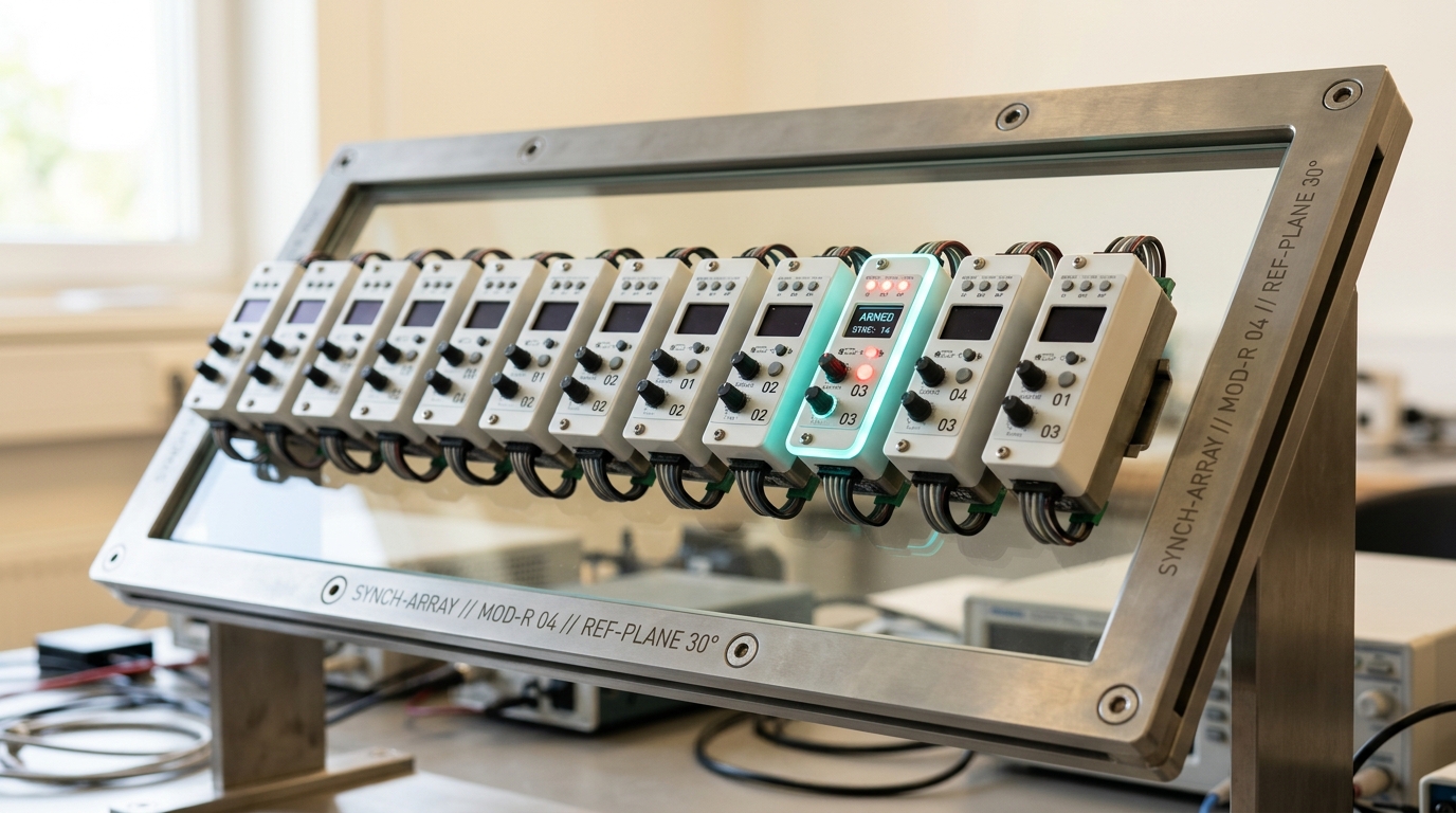
Figure 1. Simultaneity is not free. Someone has to build the plane that says which events count as "at once," and this bank of clocks is how.
This construction is not confined to flat spacetime or to elementary particles. Janson and Lopp have recently extended exactly this hypersurface-centroid bookkeeping to a composite quantum particle’s own internal structure in a curved, Schwarzschild-type background, deriving the general-relativistic corrections a multi-particle atom’s centre-of-mass coordinate picks up when the atom itself is used as a clock in an interferometer [14]. The atlas built here stays in flat spacetime throughout, but the same (u,Σ)↗ bookkeeping is what makes that curved-spacetime extension possible at all.
The scale that answer is measured against is fixed entirely by the body itself. For a system of total mass M↗ and spin angular momentum of magnitude ∣S∣↗ — the part of Jμν↗ left over once the orbital piece is subtracted — define
ρM↗ has units of length by inspection, angular momentum divided by momentum, and it is built from nothing but the two Poincaré-invariant labels, mass and spin, that every observer agrees on regardless of which chart they read a position off of. It will turn out to be the radius of the region within which every well-behaved chart in this atlas has to stay.
The Disk a Free Body Draws Around Itself
Fix the slicing convention that anchors the centroid to the body’s own rest frame — the choice, standard in the spinning-body literature, in which the spin tensor about the centroid satisfies SαβPβ=0↗ — and ask how Xμ(u,Σ)↗ moves as u↗ is varied away from the body’s own rest-frame observer to some other inertial observer boosted at velocity v↗ relative to it. Costa and Natário’s synthesis of the classical spinning-body literature gives the answer in closed form: the centroid measured by the boosted observer is displaced from the rest-frame centroid by
a shift transverse to both the spin and the relative velocity [13]. This is an exact identity of special relativity, not an approximation valid only for small v↗; it holds all the way to v→c↗, at which point ∣Δx∣→∣S∣/(Mc)=ρM↗ exactly, since ∣S×v∣≤∣S∣v↗ saturates when the spin is perpendicular to the boost. No boosted observer, however extreme, can push a body’s own centroid further from its rest-frame value than ρM↗. As u↗ ranges over every inertial observer, Xμ(u,Σ)↗ traces out a disk of exactly that radius, orthogonal to S↗ — the world-tube first identified by Møller and reproduced in modern language by Costa and Natário’s review of spin supplementary conditions [13].
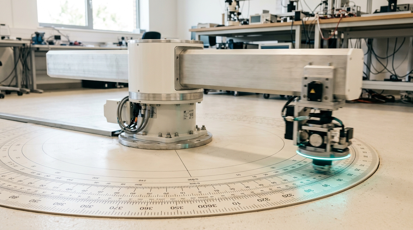
Figure 2. Every observer who circles the same body draws a point on this disk. None of them is off the disk, and none of them is at its center.
This is the atlas’s first transition function, and it is worth stating exactly what it does and does not compare. It holds the spin supplementary condition — the rule that picks out a unique centroid once an observer is specified — completely fixed, and varies only the observer. It says nothing yet about what happens if the observer is held fixed and the rule itself is changed; that is the next chart’s business. And it comes with two checks for free. First, a conservation check: Pμ↗ and Jμν↗, the body’s total four-momentum and total angular momentum, are identical for every observer in this comparison, since they are the Poincaré charges of one physical state and no relabeling of which point counts as “the centroid” touches them. Only the split of Jμν↗ into an orbital part and a spin part shifts, and it shifts by exactly the amount needed to keep Jμν↗ fixed. Second, a limiting-case check: as v/c→0↗, Δx→0↗ for every finite spin, and every observer’s centroid collapses onto the same point — the nonrelativistic, frame-independent Newtonian centroid RN↗ this article started from. That is the known-theory recovery Newtonian mechanics has every right to demand, and it is exact rather than asymptotic in some uncontrolled sense: the correction is order v/c↗ and vanishes identically at v=0↗.
A number makes the scale concrete without pretending to describe an experiment. Take a spin-one-half wavepacket of electron mass, S=ℏ/2↗, so that ρM=ℏ/(2mec)≈1.931×10−13m↗, essentially half the electron’s reduced Compton wavelength. Boost it transverse to its own spin at β=v/c=0.6↗. The exact centroid shift between the rest-frame observer and the boosted observer is
about a hundred and sixteen femtometres — smaller than a proton’s charge radius, far below anything a position-resolving instrument built from ordinary matter could hope to see directly, and yet an exact analytic evaluation of a closed-form identity, not a simulated or measured quantity. It is reported here as illustrative of the atlas’s characteristic length, nothing more.
ADVERTISEMENT
Two Centroids Cannot Both Keep Their Promises
Hold the observer fixed now, and ask what happens when the spin supplementary condition itself is changed instead of the observer. Pryce’s 1948 classification answered this before quantum field theory had settled on the machinery used elsewhere in this series: of the several ways to generalize the Newtonian centroid relativistically, most reduce to two structurally distinct families once spin is included [1].
The first, the covariant centre of energy, transforms simply as the spatial part of a four-vector under a change of Lorentz frame — exactly the property Xμ(u,Σ)↗ was built with above — but its three spatial components fail to commute with each other once spin is present, by an amount proportional to the spin itself. The second, constructed by Newton and Wigner for exactly this purpose and reproduced in Pryce’s classification as a distinct case, has strictly commuting components, [XNWi,XNWj]=0↗, the property any operator called “position” ought to have if it is to support ordinary probability densities and wavefunction localization at all, at the price of no longer transforming as a four-vector: an observer in a different inertial frame does not simply Lorentz-boost the Newton–Wigner operator into the new frame’s Newton–Wigner operator, because the two are built from a boost generator that itself carries spin-dependent, frame-tied structure [2]. Fleming’s manifestly covariant reformulation makes the trade-off explicit rather than incidental: commuting components and simple four-vector transformation cannot both be had from the same operator whenever spin is nonzero, and every choice in the literature buys one property by sacrificing the other [4].
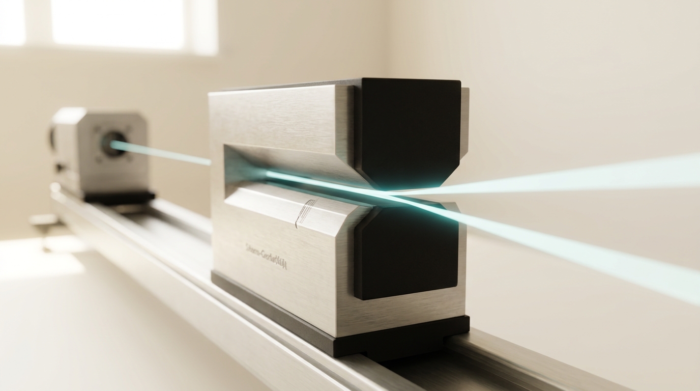
Figure 3. One magnet, one incoming beam, two answers. The two paths have not been asked to meet again yet.
The derivation behind this trade-off runs through the ten generators of the Poincaré algebra rather than through anything special to a particular particle. The boost generator K↗ is one fixed physical object for a given one-particle state; writing it as a symmetrized combination of a position candidate and the energy only closes the algebra’s commutation relations correctly if either the position candidate absorbs a spin-momentum term, yielding commuting components and frame dependence, the Newton–Wigner choice, or that term is left attached to the boost generator itself, leaving the position candidate free of it but noncommuting, the covariant choice. Both are legitimate solutions of the same algebraic constraint; neither is an error. What the two share, and what makes them members of one atlas rather than two unrelated proposals, is that both reduce to the identical operator the instant spin vanishes: at S=0↗ the noncommutativity of the covariant centroid is identically zero, the frame-dependence of the Newton–Wigner operator disappears along with the spin-momentum term that caused it, and both collapse onto the same Newtonian RN↗ this section began from — the second limiting case this atlas is required to pass, satisfied exactly rather than approximately, because the obstruction in both directions is literally proportional to S↗.
It is worth being precise about what kind of object each chart in this pairing actually is, because the two are not interchangeable answers to the same experiment. Xμ(u,Σ)↗, built from a classical or semiclassical stress-energy distribution, is a number: a spacetime point associated with one physical configuration. XNW↗ is an operator on a Hilbert space, and what a quantum experiment actually reports is not XNW↗ itself but expectation values and, eventually, click statistics built from it. The two charts answer “where is it” for two different kinds of description of the same underlying physics, classical field and quantum state, and the atlas has to keep that distinction visible rather than silently identifying an operator with a number.
A Coordinate That Shakes While Standing Still
The Newton–Wigner operator was not built for elegance; it was built to repair a specific, observable pathology in the naive Dirac position operator x^↗, the coordinate that appears literally in the Dirac equation. Because a free Dirac wavepacket generically mixes positive- and negative-energy plane-wave components, x^↗'s Heisenberg equation of motion picks up, alongside the ordinary uniform drift, an oscillating term with no classical counterpart: an angular frequency
set purely by the rest mass. For an electron this is ωZ≈1.55×10²¹rads−1↗, an oscillation period of roughly four zeptoseconds in the particle’s own rest frame — a boosted lab observer would clock a longer, time-dilated period by the ordinary factor γ↗, coordinate time and proper time parting ways in exactly the usual manner — with an amplitude of order the reduced Compton wavelength ℏ/(mec)↗, the same length scale, twice ρM↗ for a spin-half particle, that bounded the Møller disk above. Schrödinger first noticed this trembling motion, zitterbewegung, in the Dirac coordinate’s equations of motion; Foldy and Wouthuysen’s 1950 canonical transformation is what removes it, by transforming to exactly the representation in which the position operator is the Newton–Wigner operator and the oscillating term is absorbed into the difference between x^↗ and XNW↗[3].
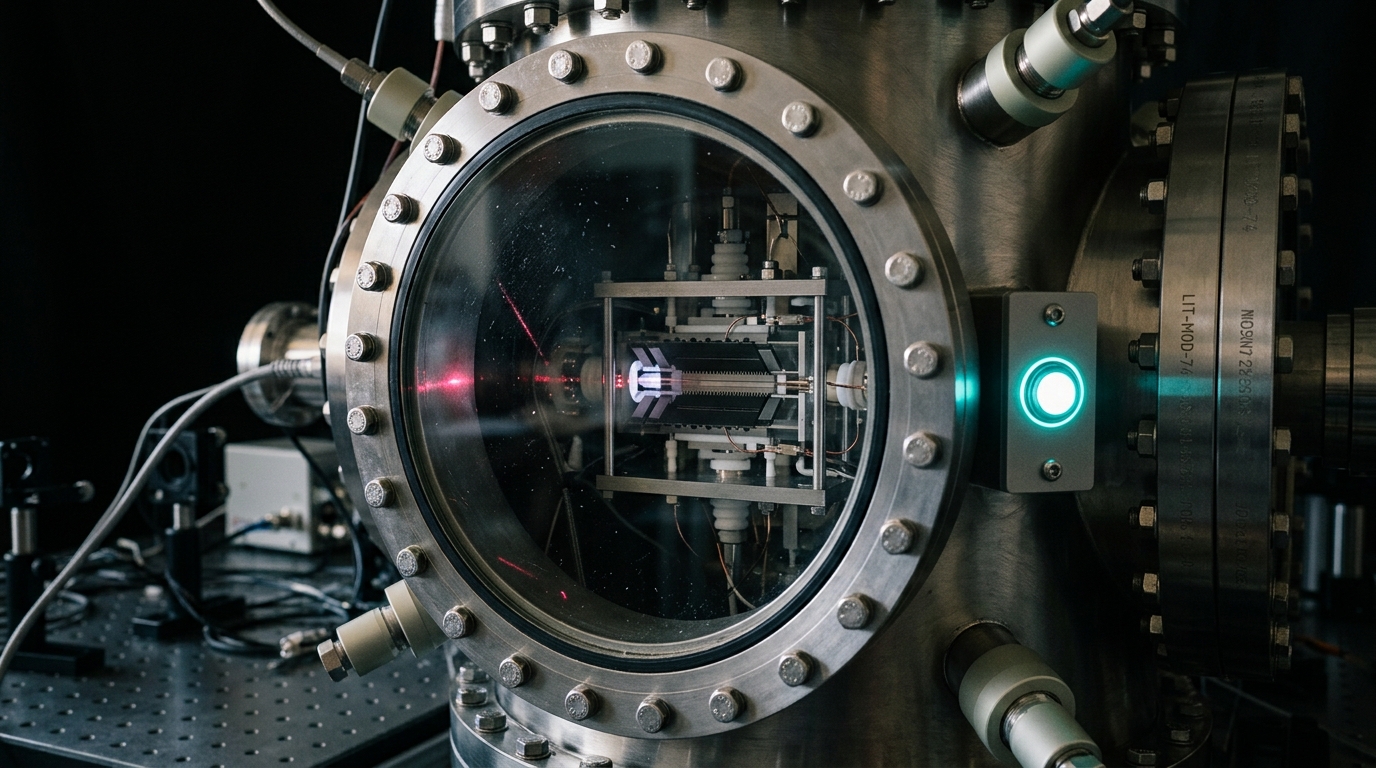
Figure 4. Something in here is being made to tremble on purpose, at a frequency no free electron will ever show a lab bench.
Zitterbewegung is not directly observable in a free electron — the effect sits at a length and time scale no free-particle experiment has resolved — but its structure has been observed exactly where it can be engineered: in a single trapped ion whose internal levels and motional states are driven to reproduce the one-dimensional Dirac equation’s own dynamics term for term. Gerritsma and coworkers built such a simulator and measured the ion’s simulated position executing precisely this oscillation, including the predicted crossover as the simulated mass parameter is tuned from relativistic to nonrelativistic [15]. That is an observed fact about an engineered quantum simulation of the Dirac equation, not a measurement of a free electron’s own trembling, and the distinction is kept explicit here rather than allowed to blur into a claim this construction has not earned.
What zitterbewegung adds to the atlas is a fourth, sharper illustration of the same structural point as the Pryce trade-off: x^↗ and XNW↗ disagree not by a fixed offset but by a time-dependent, oscillating quantity, largest exactly where a wavepacket carries significant negative-energy content, a regime the nonrelativistic limit removes entirely. As v≪c↗ and the wavepacket is restricted to the positive-energy subspace, the oscillating term’s amplitude falls relative to the packet’s own spatial width, and x^↗, XNW↗, and RN↗ converge onto one description — the same nonrelativistic recovery checked twice already, confirmed here a third time from an entirely different starting operator.
Why No Chart Covers the Whole Atlas
Every chart built so far shares an unstated assumption: that “the particle is here, now” is at least momentarily a sharp, meaningful statement, even if which “here” depends on which chart is consulted. Hegerfeldt’s 1974 theorem removes that assumption for all of them at once. Take any one-particle state with positive-energy free time evolution, the ordinary requirement that a legitimate quantum state have no negative-energy components below some fixed lower bound, and suppose it is exactly localized in a bounded spatial region at one instant, with the wavefunction identically zero outside that region. Hegerfeldt showed that under free evolution the probability of finding the particle arbitrarily far outside that region becomes strictly nonzero after any nonzero elapsed time, however short [6]. A decade later he sharpened this to a stronger and more disturbing form: a state need not even be exactly localized to begin with, only to have exponentially bounded tails, for the same instantaneous spreading beyond any finite distance to appear [7]. Perez and Wilde reached an equivalent conclusion by a different, more axiomatic route, showing that causality, translation covariance, and positivity of the energy spectrum are jointly incompatible with any notion of strict localization in a bounded spacetime region at all [8].
None of this says a relativistic particle’s position is meaningless. It says the specific combination this atlas has been building — a sharp operator, exact eigenstates, and strictly causal free-particle dynamics — cannot be jointly realized by any chart above, Newton–Wigner included. The theorem applies to XNW↗ exactly as it applies to x^↗, since commuting components buy nothing against Hegerfeldt’s argument; the argument never uses the commutator structure, only positivity of energy and the existence of a bounded region with zero amplitude outside it.
Quantum field theory sharpens the same conclusion in language that does not mention wavepackets at all. The Reeh–Schlieder theorem states that the vacuum state of a quantum field theory is cyclic for the algebra of operators localized in any bounded spacetime region, however small: acting on the vacuum with operators supported only in that small region can approximate any state in the entire Hilbert space to arbitrary precision. Witten’s survey of the theorem’s consequences makes the relevant point directly — no nontrivial local operator can annihilate the vacuum, so there is no state, in the full field-theoretic description, that is exactly and only present in one bounded region with literally nothing correlated to it everywhere else [10]. Sharp localization is not merely hard to achieve with the charts built above; it is foreclosed at the level of the algebra those charts are built out of.
This is the atlas’s genuine boundary, not a gap waiting on a cleverer construction. Every chart from the Newtonian centroid through the Newton–Wigner operator is a legitimate, checkable answer to “where, approximately, and according to which convention,” and every one of them stops being exactly true, in the strict sharp-operator sense, the instant it is pushed to describe a state confined with certainty to a bounded region and evolving causally. The next chart exists because of this limit, not despite it.
Trading a Sharp Line for a Blurred Detector
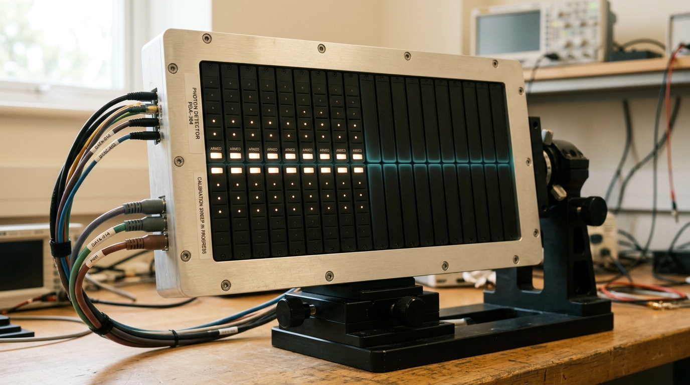
The response to Hegerfeldt’s obstruction that has actually held up is to stop asking for a sharp position operator at all. Werner’s screen observables replace the eigenvalue-and-projector structure of x^↗ or XNW↗ with a positive-operator-valued measure: a family of positive operators, one for each region of a detection screen, that sum to the identity and assign a probability to “a click registered in this region” without ever claiming the particle possessed a definite position immediately beforehand [9]. A POVM chart is a genuinely different mathematical type from every chart built so far, not a self-adjoint operator with a spectral decomposition into sharp positions but a measure-valued object whose value on any given trial is a probability distribution over an actual detector’s actual geometry. It sidesteps Hegerfeldt’s theorem because it never asserts exact localization to begin with; its resolution is set by the physical smearing of the detection scheme rather than driven to zero by fiat, and the causality argument that dooms a sharp projector has no state to act on that it can call “exactly here.”
Figure 5. This screen was never going to report a point. It reports which cell answered, and that is the whole of what it can honestly promise.
This chart is not optional window-dressing kept in reserve for elegance; for one important class of particle it is the only chart available. Wightman’s 1962 analysis of localizability by irreducible representation of the Poincaré group established that a genuine, covariant, Newton–Wigner-type position operator exists for every massive representation, of any spin, but fails to exist for massless representations of helicity magnitude one or greater [5]. The photon is exactly such a representation. There is no covariant chart of the earlier kind, and no Newtonian rest-frame chart either, since a photon has no rest frame to define one in. Every sharp chart this atlas has built so far has a missing page precisely where light itself would be entered. What remains for a photon is the operational chart: a detector screen, a POVM, and a click.
That gap is not a defect unique to this construction; it is the reason “where is a photon” has always been treated more gingerly in the literature than “where is an electron.” It also explains, in advance, why the experiment taken up next has to be read as an operational measurement rather than as a report on any operator’s eigenvalue: light was never going to answer through the earlier machinery, because that machinery was never built to accept it.
A Postselected Estimator That Owes the Map Nothing
There is a fifth kind of answer to “where,” and it is worth stating precisely how it differs from all four above before using it. Prepare a system in a state ∣ψ⟩↗, couple it weakly to a pointer, and then postselect on a final state ∣f⟩↗ measured after the coupling. The weak value of any observable A^↗, position among them, conditioned on that postselection is
introduced by Aharonov, Albert, and Vaidman as the quantity a weakly coupled pointer’s mean shift actually reports, to leading order in the coupling strength, once the postselection has been performed [11]. Aw↗ is not an eigenvalue of A^↗, not an expectation value in the ordinary sense, and not guaranteed to be real: it is built from an amplitude ratio over a sub-ensemble selected by an event, the postselection, that has not yet happened at the time the weak coupling acts.
An exact two-level calculation shows how far this can depart from the intuitive picture. Preselect a spin-one-half system along x↗, ∣ψ⟩=21(∣↑⟩+∣↓⟩)↗, and postselect along y↗, ∣f⟩=21(∣↑⟩+i∣↓⟩)↗. Then ⟨f∣ψ⟩=21(1−i)↗ and ⟨f∣σz∣ψ⟩=21(1+i)↗, so the weak value of σz↗ is
σz↗ has eigenvalues ±1 only, yet its weak value here is purely imaginary, not merely outside the eigenvalue range but off the real line entirely. This is an exact, closed-form evaluation of the defining ratio, not a measured or simulated number, stated here only to make concrete what “anomalous weak value” means before the same word is applied to a spatial coordinate rather than a spin component.
Applied to position, the same object, xw=⟨f∣x^∣ψ⟩/⟨f∣ψ⟩↗, is this atlas’s fifth chart, and it is admitted with a label the other four do not carry. xw↗ answers a genuinely different question from every chart above: not “what does this state’s position operator return,” but “what does a weakly coupled pointer’s mean reading become, once conditioned on an event that filters the ensemble after the fact.” Because the conditioning can make ⟨f∣ψ⟩↗ arbitrarily small, xw↗ can be pushed arbitrarily far from anything the Møller disk or the Pryce trade-off constrains; it is not bounded by ρM↗, and it does not need to be, because it was never built from the operational protocol that produced the ρM↗ bound in the first place. An anomalous weak value lying outside the disk this atlas draws for its sharp charts is not a contradiction, because comparing it directly to those charts as though it answered the same question would be exactly the mismatched-protocol error this construction is built to catch, not commit. For that reason no disagreement number is computed here between xw↗ and XNW↗ or Xμ(u,Σ)↗; the honest statement is that the comparison is not defined, not that it has been evaluated and found large.
Light Has No Business Being Where the Data Put It
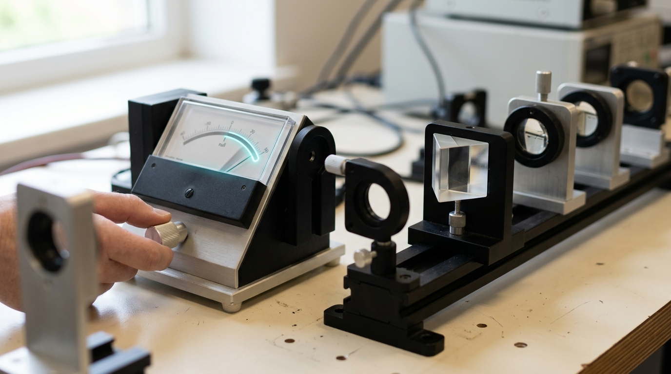
The one place any of this touches an actual measured number is optical, not electronic, and it arrives through the weak-value chart rather than through any operator eigenvalue. Light crossing an interface between media of different refractive index acquires a transverse, polarization-dependent displacement, the spin Hall effect of light, far smaller than the beam’s own wavelength under ordinary detection. Hosten and Kwiat used exactly the weak-value amplification structure above, preselecting the photons’ polarization and postselecting on a nearly orthogonal state, to enhance the effective displacement by close to four orders of magnitude and resolve a shift at the angstrom scale [12]. What was measured is a pointer’s mean shift, exactly the Aharonov-Albert-Vaidman quantity, not a photon’s position eigenvalue; the amplification is a direct laboratory instance of a weak value being made large by pushing the postselection toward orthogonality, the identical mechanism behind the imaginary σz↗ value computed above.
Figure 6. The shift this bench is built to catch is smaller than the light's own wavelength. Amplifying a small number honestly is a discipline, not a trick.
The connection to the rest of this atlas is not merely thematic. Harte and Oancea showed that the equations governing a light beam’s spin-dependent trajectory in a medium with a varying refractive index are a special case of the Mathisson–Papapetrou equations that govern a classical spinning body’s centroid motion, the same equations behind the Møller disk in the second section of this article [16]. The spin Hall effect of light is, in this sense, a Møller-type centroid shift for a massless spinning ray, computed and observed in a regime where no covariant Newton–Wigner-type operator underlies it, because Wightman’s result had already forbidden one for a helicity-one representation. What is actually pulled out of the data, though, is not that classical centroid directly but a weak value amplifying it into visibility. The one experiment in this atlas with a real number attached sits at the intersection of three charts at once — the Mathisson–Papapetrou centroid supplying the physical effect, the missing covariant operator explaining why light needed a different route to it, and the postselected weak value providing the only route that worked — and that intersection, not any single clean chart, is where the laboratory currently lives.
What the Atlas Keeps, and Where It Runs Out of Paper
Collect the pieces. Three charts, the Newtonian centroid RN↗, the observer-dependent stress-energy centroid Xμ(u,Σ)↗, and the canonical Newton–Wigner operator XNW↗, form a genuine, well-behaved sub-atlas. Define, for any two of them evaluated on the same hypersurface Σ↗,
the proper spatial separation within Σ↗ between the two charts’ answers, normalized by the spin-to-mass length fixed in the first section. δij↗ is dimensionless by construction, symmetric, zero exactly when the two charts coincide, and it has now been checked, not merely asserted, in both directions this kind of construction is required to pass: it vanishes as v/c→0↗ for any spin, and it vanishes as S→0↗ for any observer or Lorentz frame. It is bounded above by exactly 1 for the observer-transition case, since ∣Δx∣≤ρM↗ was shown above to saturate rather than merely approach that value. Both checks are this construction’s kill criterion, run rather than assumed: had either limit failed to collapse the disagreement to zero, the atlas would have been reporting confusion between an artefact of convention and an artefact of mismatched apparatus, exactly the failure this kind of object is meant to be judged by.
What none of these three charts ever disputes is Pμ↗ and Jμν↗, the body’s total four-momentum and total angular momentum, the two Poincaré charges no relabeling of “centroid” touches. Every version of “where” argued about above is a statement about how Jμν↗ is split into an orbital part and a spin part; the sum is never in question. That is the single invariant this entire atlas, sharp and operational charts alike, is built on top of: physics agrees completely on what the body has, mass, momentum, energy, and spin, and only argues about which point should be credited with carrying the orbital share of the angular momentum.
The fourth and fifth charts, the postselected weak value and the detector-tied POVM, are not extensions of that same sub-atlas; they are a different kind of object answering a different kind of question, and the honest finding here is that the atlas does not close around them. Hegerfeldt’s theorem and its axiomatic restatement by Perez and Wilde forbid gluing a sharp, causally propagating position operator onto the free-particle dynamics any of these charts assumes; the Reeh–Schlieder theorem forbids it again, more severely, at the level of the field algebra itself. The POVM chart exists because the sharp charts cannot be pushed past that limit, not because someone chose it for convenience, and for a photon, a helicity-one representation with no Newton–Wigner operator to begin with, it is not a fallback option but the only chart on offer. The weak value, meanwhile, is permitted to leave the ρM↗ disk entirely, without contradiction, precisely because it was never built from the protocol that disk was derived for.
An atlas, in the geometer’s sense, is a set of charts whose transition functions agree wherever the charts overlap. The first four sections of this one satisfy that definition exactly, with an explicit, exactly derived transition function and two independently checked limits. The sections after do not extend it; they mark where it stops, for reasons that are theorems, not oversights. A relativistic position was never one point waiting to be found more carefully. It is a small number of exactly comparable charts, a length scale that bounds their disagreement, and a boundary, proven rather than assumed, past which the word stops referring to a point at all — and the one real number this article touched, an angstrom-scale shift pulled out of ordinary light at an ordinary glass surface, was found exactly there, on the side of that boundary where a sharp answer was never going to be available.
Share this Article
Pass along these insights to your network across your favorite platforms.