A detector clicks; a theorist calls it a particle. Between those two events sit four matching conditions nobody checks by default. This program builds the distance that prices a mismatch, and finds one case where the distance itself will not compute.
Research paperRevolutionary Life 75, Series D, No. 5 ·
this page is the paper's summary — the full text is the PDF.
Download the paper (PDF)
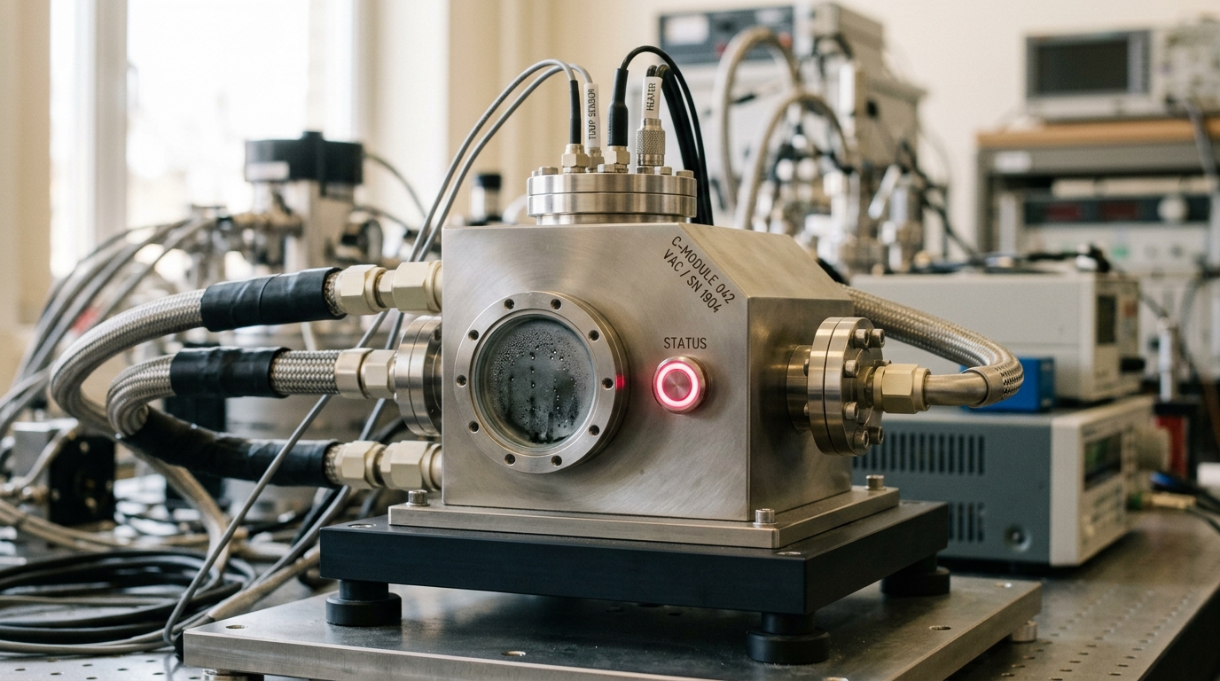
Two worldlines, two records of the vacuum. Whether they are reporting the same thing is not a philosophical question once the cables are plugged in.
Abstract
Whether the vacuum contains a particle is not settled by the field alone; it depends on the worldline used to decompose the field into modes, an ambiguity fixed by Bogoliubov coefficients and sharpened by the Unruh effect. This article treats that dependence operationally, through the Unruh-DeWitt detector's response functional rather than mode counting. It defines a total-variation distance between the normalized excitation spectra two prepared detectors report, states the four conditions -- field state, coupling type, gap, switching profile -- that must be matched before a nonzero distance can be blamed on the worldline rather than mismatched apparatus, and checks the distance is a genuine metric. It recovers the exact Planckian Unruh spectrum in the eternal-acceleration limit, derives an exact leading-order coefficient from a Wien-type transcendental equation, and finds a boundary case, the eternal inertial trajectory, where the construction's own normalization fails outright. A storage-ring polarization bound marks the only regime any of this nears a measurement. This is a derivation, not a simulation, and no click here was counted.
ADVERTISEMENT
No Particle Without a Cosigner
A photon detector clicks. Nobody disputes the click; it is a macroscopic, recorded, irreversible fact about a piece of hardware. What is not a fact of the same kind is the sentence that usually follows it: “a particle arrived.” That sentence requires a second act — a choice of which modes of the quantum field count as the ones a particle can occupy — and two observers who disagree about that choice can each build a perfectly consistent bookkeeping in which the other one’s particle simply is not there. This is not a controversial fringe claim. It is textbook physics, established since the early 1970s and demonstrated most sharply by the Unruh effect: an observer at rest in the ordinary vacuum sees nothing, while an observer undergoing uniform proper acceleration through the very same field state reports a bath of thermal particles at a temperature set by nothing but their own acceleration [1, 2]. Both observers are right. Neither is measuring a property of the field alone.
What follows is not a proposal to fix that ambiguity — it cannot be fixed, and no result below tries to. It is a proposal to make the ambiguity operational: to replace the question “is there a particle?” with a question that has a definite, checkable, numerical answer — “how much do two specific detection setups disagree, once every condition except the trajectory has been pinned down?” A particle, on this reading, is not a fact about the field. It is closer to a treaty: a claim two parties — a quantum field in a given state, and a worldline carrying a detector through it — arrive at jointly, and only after every term of the agreement other than the trajectory itself has been fixed identically for both. The object built here measures what is left over when that agreement is tested. Sometimes the leftover is a clean, calculable number. In at least one case worked out below, the object refuses to return a number at all, and that failure is as informative as any of the successes.
What a Click Has Always Meant, and What It Has Never Meant
The precise, non-negotiable content of the ambiguity is the Bogoliubov transformation. Given two ways of splitting a free field into positive- and negative-frequency modes — two choices of “particle,” in the ordinary sense of excitations above a chosen vacuum — the annihilation operators of one decomposition mix the creation and annihilation operators of the other:
When any of the coefficients βjk↗ is nonzero, the vacuum of the a↗-decomposition is a many-particle state of the a~↗-decomposition, and vice versa: “how many particles are present” is a question whose answer depends on which set of modes was declared fundamental, not on the field configuration by itself. Fulling showed this could happen already in flat, static coordinates on two-dimensional Minkowski space, purely from a nonstandard but perfectly legitimate choice of time coordinate [2]. Davies showed the same mixing follows Hawking’s black-hole derivation into the Rindler wedge of ordinary flat spacetime, associating a temperature with the horizon an accelerated observer drags behind them [3]. Unruh completed the argument with a model of the measuring device itself, not just the modes: a idealized two-level system, linearly coupled to the field along its own worldline, responds to whatever the field is doing along that specific worldline, and along a uniformly accelerated worldline in the ordinary vacuum it responds exactly as though bathed in real thermal radiation at temperature kBTU=ℏa/(2πc)↗[1]. None of this is proposed here. All of it is the baseline the rest of this article stands on.
The detector, not the mode decomposition, is the object this article works with, for a reason that matters later: a detector’s response is what an experiment can actually report, while “the Bogoliubov coefficients of the true vacuum” is not the kind of thing any apparatus reads off a dial. The response functional for a pointlike, linearly coupled two-level (Unruh-DeWitt) detector on worldline x(τ)↗, parametrized by its own proper time τ↗, with energy gap Ω↗ and switching function χ(τ)↗ controlling when the interaction is on, is
where W↗ is the field’s two-point Wightman function evaluated along the trajectory [5]. Three things in this expression are worth fixing in the reader’s mind before anything else happens to it. First, τ↗ is proper time — the detector’s own clock, the only time variable with unambiguous physical meaning for a single worldline — never the coordinate time of whatever chart the trajectory happens to be written in. Second, Ω↗ is conjugate to that same proper time; it is an energy gap measured in the detector’s own instantaneous rest frame, not a coordinate-frame frequency. Third, the field state enters only through W↗, and changing the field state — the ordinary vacuum, a thermal state, the Boulware, Hartle-Hawking, or Unruh state of a black-hole exterior — changes Fx↗ even for a fixed trajectory. Keeping these three inputs — proper time, proper-frame gap, and field state — cleanly separated is what prevents an ordinary coordinate-time effect, like gravitational redshift between two static observers at different heights, from being mistaken for a genuine disagreement about particle content. A redshift is a fact about clocks. A response-spectrum disagreement, once clocks are correctly accounted for, is a fact about the field and the worldline together.
Figure 2. The gap is the only number this module is allowed to have an opinion about. Everything else belongs to the worldline.
Unruh and Wald pushed the operational reading one step further by asking what a click actually costs: when an accelerated detector reports absorbing a Rindler-frame particle, an inertial observer watching the same event must describe it as the detector spontaneously emitting a Minkowski-frame photon, with energy conservation and causality both intact once the accelerating agent’s own work is included in the ledger [4]. A click is real. What the click means is observer-dependent, and the two descriptions are not in conflict — they are two accountings of the same energy-momentum transfer, agreeing on everything except which vocabulary, “absorption” or “emission,” gets used. That is the precedent for everything constructed below: build the comparison at the level of the click, and let vocabulary be sorted out afterward.
Four Terms Before Any Disagreement Counts
Fx(Ω)↗, viewed as a function of Ω↗ for fixed everything else, has a natural reading as a spectrum: it says how much excitation probability accumulates at each possible gap, for a whole notional bank of detectors sharing one trajectory, one switching profile, and one field state, differing only in Ω↗. Restricting to the excitation branch Ω>0↗ — “did this detector behave as though it absorbed a quantum” is the only branch this article treats as bearing on particle content, since the decay branch Ω<0↗ mixes genuine field structure with detector-specific spontaneous-emission physics that is present even in flat, empty spacetime with no field excitation at all — normalize:
defined whenever the denominator is finite and nonzero. Given two such normalized spectra, for a detector on worldline x↗ and a detector on worldline y↗, define their disagreement as the total variation distance between the two probability densities:
This is the object this article is actually about, so its bookkeeping has to be stated in full before any number is produced. Ddet↗ is a map from pairs of “treaty configurations” — worldline, field state, coupling type, and the gap/switching pair used to build the spectrum — to the real interval [0,1]; it carries no physical units, because it is built entirely from normalized probability densities over Ω↗, whose own units of inverse time cancel between numerator and denominator of every term in the integral. It inherits, rather than assumes, the property of being a genuine metric — non-negative, symmetric, zero exactly when px=py↗ almost everywhere, and satisfying the triangle inequality — because total variation distance is a metric on probability measures as a matter of elementary measure theory, independent of anything physical being fed into it. That inheritance is itself a check worth stating plainly: an ad hoc “difference score” invented for this article would need its metric properties verified by hand; Ddet↗ gets them for free because it was built from an object mathematics already understood.
Two invariances follow immediately, and one does not. Ddet↗ does not change if a trajectory is described using a different auxiliary curve parameter before being converted to proper time — proper time itself is not a gauge choice, it is the arc length of the worldline, fixed by the metric once the trajectory and the metric are fixed, so there is no freedom here to exploit. Ddet↗ also does not change under a Poincaré transformation applied identically to both worldlines and to the field vacuum together, since W↗ is Poincaré invariant and τ↗, Ω↗, and χ↗ are all defined intrinsically along each worldline. What does change Ddet↗, and is meant to, is any actual physical difference between the two setups. The discipline this article insists on is separating that meant-to variation from an unmeant one: before attributing a nonzero Ddet(x,y)↗ to “the worldlines disagree about particle content,” four other things have to be checked as identical between the two detectors, because each one moves Ddet↗ on its own, with nothing to do with x↗ or y↗ as trajectories through spacetime.
The first term is the field state — the same vacuum, or the same thermal state, or in curved spacetime the same choice among the Boulware, Hartle-Hawking, and Unruh states, since none of those is fixed by the geometry alone. The second is the coupling type: a detector linearly coupled to the field itself and a detector coupled to the field’s proper-time derivative are different instruments on the same worldline, and their response spectra carry different powers of Ω↗ in the numerator even for identical trajectories — Moustos showed exactly this, that a detector’s early-time response depends on which bilinear of the field it couples to, even though, remarkably, its late-time asymptotic state does not [9]. The third is the gap Ω↗ itself, or more precisely the requirement that Ω↗ be defined against each detector’s own proper time rather than against a shared coordinate time — two detectors at different heights in a static spacetime, or moving at different speeds, experience the same coordinate-time interval as different amounts of proper time, and building Ω↗ from coordinate time instead of proper time would inject that redshift directly into Ddet↗ as a spurious “particle disagreement” that is really just two clocks running at different rates. The fourth is the switching profile χ(τ)↗: its total duration and its smoothness both leave fingerprints in Fx(Ω)↗ that have nothing to do with the trajectory, as the next two sections show in detail.
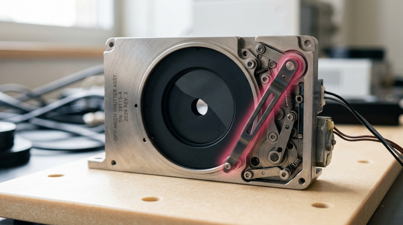
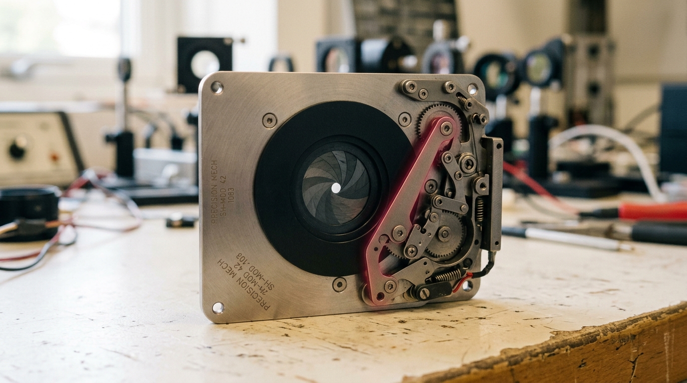
Figure 1. A detector is not always listening. The shutter is the physical fact behind the switching function, and this one has not finished closing.
These four terms are the treaty’s clauses. They are not decoration on the definition of Ddet↗; they are the difference between a number that means something about spacetime and a number that means something about laboratory bookkeeping. A nonzero distance computed without matching all four is not evidence about worldlines. It is evidence that two different instruments were used, which is a true but uninteresting thing to discover.
Where the Spectrum Settles Into a Known Answer
The first check any new object owes the literature is that it reproduce the literature’s own answer in the case the literature has already solved. For a worldline held at constant proper acceleration a↗ forever, coupled linearly to a massless scalar field in the ordinary vacuum, with the switching left on for all time, the Wightman function depends only on the proper-time separation and the standard Fourier transform is exact and textbook: the excitation-branch rate per unit proper time takes the Bose-Einstein form
with the proportionality constant fixed by the detector’s coupling strength and dimension — irrelevant here, since it cancels the instant the spectrum is normalized [1, 5]. Takagi confirmed the same detailed-balance structure holds for a Rindler wedge of any spacetime dimension, which rules out the possibility that the thermal form is some low-dimensional accident of the four-dimensional calculation [7]. This is exactly the Planck spectral shape at temperature TU=ℏa/(2πckB)↗, recovering the Unruh temperature as this article’s known-theory baseline, not as anything new.
Two worldlines held at accelerations a1↗ and a2↗ therefore differ only by which Planck-shaped curve their normalized spectrum traces, and identical accelerations trivially return Ddet=0↗ — the reparametrization check every metric has to pass, satisfied here for the most literal reason available: identical trajectories are, in fact, identical.
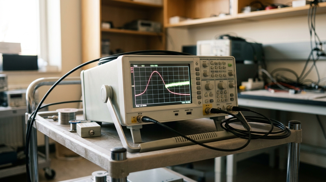
Figure 4. Two spectra, one comparison. The distance between them is not read off a screen; it is computed after the sweep finishes, and this sweep has not.
A second limit worth naming, because it is where the eternal-acceleration answer above starts to strain, is slow time dependence. Barbado and Visser worked out the response of a detector whose acceleration a(τ)↗ varies with proper time, expanding in powers of a˙↗, a¨↗, and higher proper-time derivatives of the acceleration [8]. At leading order, wherever the acceleration changes slowly compared to the local orthogonalization timescale it sets for itself, the detector reports the instantaneous Unruh temperature TU(a(τ))↗ at each moment, as though briefly and locally eternal. This adiabatic recovery is the second known limit this construction inherits rather than derives: it says Ddet↗ between a strictly eternal trajectory at acceleration a↗ and a slowly varying trajectory that happens to pass through a↗ at some instant should vanish to leading order in the rate of change, with corrections controlled by exactly the jerk and snap terms Barbado and Visser compute.
The Draft That Never Gets Ratified
The natural next question is what happens at the opposite extreme from uniform, eternal acceleration: an inertial detector, held in the same eternal, unswitched limit, in the same ordinary vacuum. Here the construction runs into a genuine wall, and it is worth walking through exactly where, because the failure is instructive rather than a rounding error.
An inertial worldline’s Wightman function is the flat-space, two-point function of the free vacuum, whose Fourier transform against e−iΩΔτ↗ has support only for Ω<0↗ — this is nothing more exotic than vacuum stability, the same textbook fact that says an unaccelerated atom in its ground state, coupled to the electromagnetic vacuum, never spontaneously jumps up in energy [6]. Consequently F˙inertial(Ω)=0↗ identically for every Ω>0↗, not approximately, not in some limit — exactly zero. The normalization integral ∫0∞F˙inertial(Ω′)dΩ′↗ is therefore also exactly zero, and pinertial(Ω)↗ is 0/0: undefined.
This is not the same kind of zero-over-infinity problem that shows up when comparing two accelerated trajectories, and the difference matters. For an eternal accelerated trajectory, both the numerator and the denominator of the naive, un-normalized response functional are proportional to the (formally infinite) total elapsed proper time, and that shared infinity cancels cleanly in the ratio, which is exactly the standard trick — divide the total accumulated response by the total proper time elapsed — used throughout this literature to extract a finite rate from an eternally switched-on detector. For the eternal inertial trajectory, the numerator does not merely fail to diverge fast enough to survive the ratio: it vanishes on the nose, for every gap, at every order. There is no shared infinity to cancel against, so there is nothing left for the ratio trick to rescue. Ddet↗ against an inertial comparison worldline in this idealized limit is not small. It is not defined.
Figure 5. Nothing arrived on this arm. Silence is a legitimate reading, but it is not a spectrum, and it cannot be normalized into one.
The honest reading of this is not that the inertial case is somehow paradoxical — physically, nothing is wrong: an inertial detector in the vacuum, left on forever, simply never clicks on the excitation branch, which is exactly the statement that the vacuum is empty from an inertial point of view. The failure belongs to the mathematical object Ddet↗, not to the physics it is trying to summarize. A distance between two probability distributions cannot be computed when one of the two distributions does not exist. The fix available is the one the switching-function literature already worked out for a related reason: give the inertial detector a finite switch-on, so that transient, non-eternal excitation probability appears even where the eternal limit gives none. Louko and Satz showed that switching on and off necessarily produces exactly this kind of transient content, and that if the switching is not smooth — a sharp step rather than a gradual ramp — the instantaneous transition rate develops a logarithmic divergence right at the switching instants, an artifact of the switching function’s own discontinuous derivative rather than any statement about the trajectory [10, 11]. Their fix — smoothing the switch, or regularizing with a spatial profile — restores a finite, comparable spectrum, but at the cost of making Ddet↗ depend explicitly on how the switching was smoothed, which is precisely the fourth treaty clause reasserting itself: match the switching profile, not merely its duration, or the comparison is measuring the shape of the shutter rather than the shape of spacetime.
The verdict this section owes the reader plainly: in the case that looks like the cleanest possible test of the Unruh effect — perfectly eternal, perfectly inertial versus perfectly eternal, perfectly accelerated — the construction proposed here cannot be made to return a number without an additional choice (a finite switching profile) that the eternal limit was specifically trying to avoid needing. This is a real boundary of the construction, not a technicality to be footnoted away, and it is reported here because the addendum governing this kind of paper is right that a mathematical object earns trust partly by admitting where it breaks.
How Far Two Signatories Can Drift
Where Ddet↗ is well defined, it can be evaluated, and the cleanest case where it is well defined and non-trivial is a comparison between two accelerated trajectories, both with finite normalizable spectra, differing only slightly in acceleration. This is the one calculation in this article carried to an explicit number, and it is carried out by hand, exactly, as a leading-order (linear-response) expansion — not a simulation, and not a claim about any measured system.
Write the normalized accelerated spectrum in terms of the dimensionless ratio u≡cΩ/a↗, using the exact Bose-Einstein shape derived above. Carrying out the normalization integral, ∫0∞Ω(e2πcΩ/a−1)−1dΩ=a2/(24c2)↗, using the standard result ∫0∞x(ex−1)−1dx=π2/6↗, gives the scale-family form
Every accelerated detector’s normalized spectrum is the same universal curve g↗, only rescaled by a/c↗. For two accelerations separated by a small increment, a↗ and a+δa↗, standard calculus for a scale family gives, to leading order in δa↗,
This is the same trick used to derive Wien’s displacement law: because ug(u)↗ rises from zero, passes through a single interior maximum, and falls back to zero, the integral of the absolute value of its derivative over all u↗ is exactly twice that maximum, with no need to evaluate the integral directly. Finding the maximum of ug(u)=24u2/(e2πu−1)↗ means solving e2πu(1−πu)=1↗, the same class of transcendental equation that fixes the peak of a Planck spectrum weighted by an extra power of frequency. Solved by Newton’s method to five-figure precision, the nontrivial root is u∗≈0.25363↗, at which u∗g(u∗)≈0.3937↗. The leading-order sensitivity is therefore
Two accelerated worldlines whose accelerations differ by one part in a thousand disagree, on this measure, by about four parts in ten thousand in normalized excitation content — a small number, appropriately, since a one-part-in-a-thousand physical difference should produce a comparably graded disagreement rather than a large one. This is the sense in which the coefficient 0.394 is an exact result: it is the exact leading term of a convergent expansion in δa/a↗, obtained from an exact closed-form spectral shape by ordinary calculus, with the only numerical step being the solution of one transcendental equation to a stated precision. It is illustrative, not a report of anything measured, and it says nothing about accelerations that are not small perturbations of one another.
Figure 6. How far can two nearly identical accelerations drift apart before the spectra notice? The gauge in this rig is the honest way to ask.
A second, purely structural check follows from the same shape function without any new arithmetic. Because a derivative-coupled detector’s response carries higher powers of Ω↗ in its numerator than a monopole-coupled detector’s does — the two instruments filter the same field differently, as Moustos’s coupling-type comparison already established [9] — their normalized spectra are provably different functions of Ω↗ pointwise, even on the identical worldline at the identical acceleration. Two distinct, non-coincident probability densities have nonzero total variation distance between them as a matter of definition, with no integral needing to be evaluated to know this. So Ddet↗ between a monopole-coupled and a derivative-coupled detector on the same trajectory is strictly positive — exactly the “unmatched apparatus” failure mode the treaty’s second clause exists to catch, demonstrated here in closed form rather than merely asserted.
A Curved Table, Same Rules
Nothing about Ddet↗'s definition requires flat spacetime; the response functional is written in terms of the Wightman function and proper time, both of which are perfectly well defined along a stationary worldline in a curved, static exterior. What changes in curved spacetime is that the field state is no longer unique even after the geometry is fixed: a Schwarzschild exterior supports the Boulware vacuum (empty at infinity, singular at the horizon), the Hartle-Hawking state (thermal everywhere, matching a black hole in equilibrium with its own radiation), and the Unruh state (matching outgoing Hawking flux with no incoming radiation), and a detector’s response depends on which of the three it is placed in — reinforcing, rather than complicating, the first treaty clause.
Hodgkinson, Louko, and Ottewill computed exactly this kind of comparison already, without reference to Ddet↗ as such: a static detector held at fixed areal radius and a detector on a circular geodesic at the same radius, both coupled identically to a massless scalar field, across all three vacuum states [12]. Their numerical results show response spectra that differ measurably between the static and circular-geodesic cases at the same radius and in the same vacuum state — a real, already-established instance of exactly the comparison this article’s construction was built to summarize in one number. No new curved-spacetime calculation is performed here; the honest claim is narrower and more useful: Ddet↗, applied to their published spectra, gives a single figure of disagreement where the source material reports whole curves, and the treaty language developed above gives a name to the four conditions their comparison already had to hold fixed — same field state, same coupling, same locally measured gap, same switching — to make that disagreement mean something about the difference between hovering and orbiting rather than about mismatched detectors.
The Only Table Where Anyone Has Actually Sat Down
Every calculation above concerns idealized, exactly solvable trajectories. It is worth being direct about how far that is from anything an experiment has touched, and the one place a real, if imperfect, physical analogue exists is worth stating with its caveats attached rather than left as an implication.
Electrons circulating in a storage ring undergo enormous proper acceleration — for an ultra-relativistic beam of Lorentz factor γ↗ on a ring of radius r↗, the proper centripetal acceleration is a≈γ2c2/r↗. For beam parameters typical of a large electron-positron collider, with γ↗ of order 2×10⁵ and r↗ of order several kilometers, this works out to a∼8×10²³ms−2↗, corresponding by the Unruh formula to TU=ℏa/(2πckB)∼3×103K↗ — a temperature scale that is, remarkably, not astronomically small, unlike the roughly 10−19K↗ an Earth-bound laboratory accelerometer would need a planet’s worth of gravity to approach. Bell and Leinaas pointed out that the relevant observable is not a literal thermometer reading but the equilibrium spin polarization of the circulating electrons, set by the competition between synchrotron-radiation spin-flip transitions (the Sokolov-Ternov effect) and any Unruh-like depolarizing correction sourced by the acceleration itself [13].
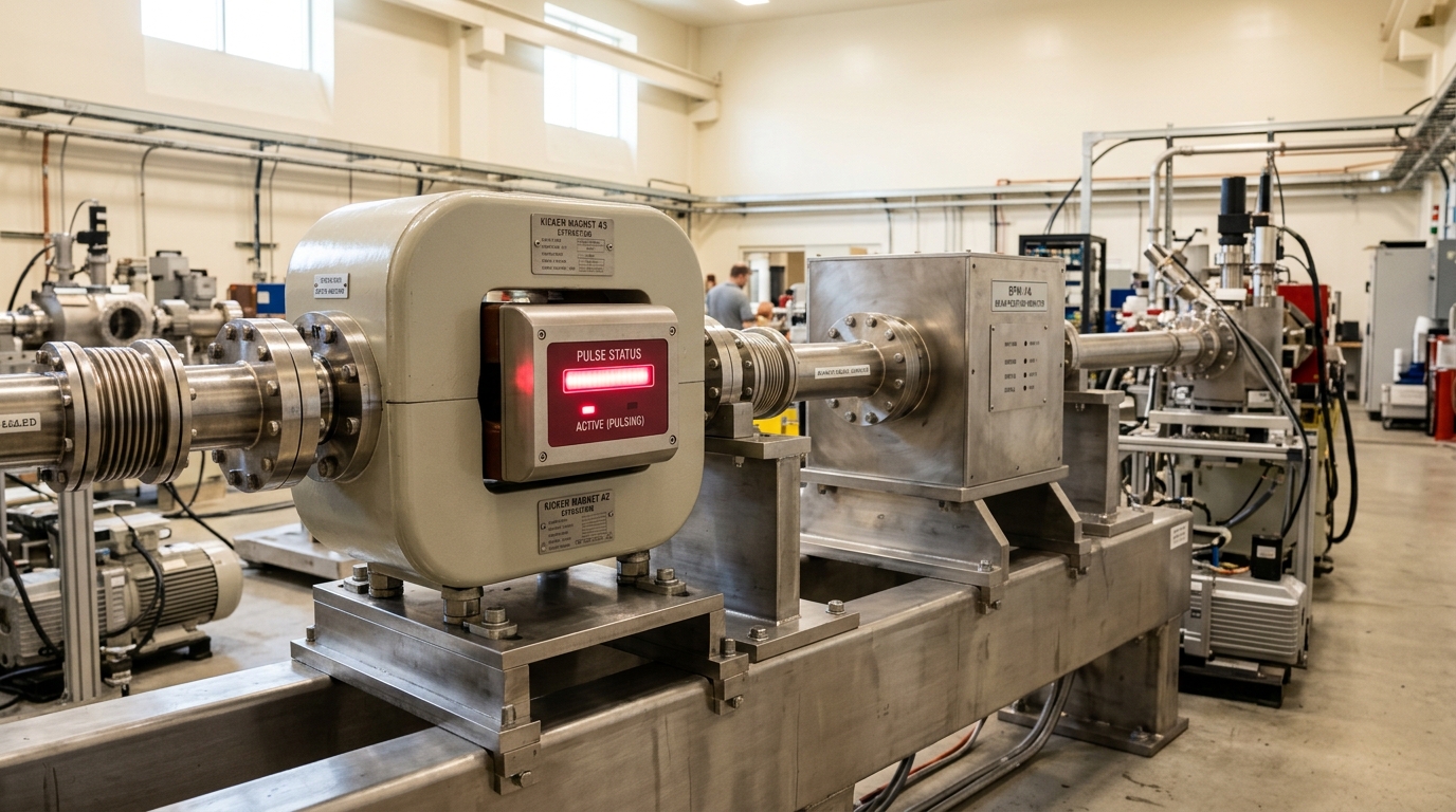
Figure 3. This is the one rail in the whole set that has actually carried a charge. Everything upstream of it is still argument, not data.
No experiment has isolated an Unruh-like signal from this system, and this article does not claim otherwise. Measured storage-ring polarizations match the standard Sokolov-Ternov prediction, once ordinary QED corrections are included, at the percent level, and circular motion is not uniform linear acceleration — a fact Bell and Leinaas themselves stressed, since the field seen by a circulating charge is not simply a Rindler wedge, and the comparison to Ddet↗'s idealized eternal-linear-acceleration spectrum is only approximate even before synchrotron backgrounds are considered. What the storage-ring case does supply, honestly, is a parameter range: it is the one setting where the acceleration scale entering TU↗ is large enough for an Unruh-like correction to be even nominally comparable to measured precision, and the percent-level agreement between observed and standard-model-predicted polarization bounds any anomalous, acceleration-induced departure from ordinary detector response at that same percent level in this one geometry. Every other trajectory discussed in this article — flat-space uniform acceleration at laboratory-achievable scales, curved-spacetime stationary orbits — sits at accelerations many orders of magnitude below where any such bound has ever been tested.
Terms No Treaty Fixes
Collect what has actually been shown, and what has only been proposed. That a Bogoliubov transformation mixes particle content between mode decompositions, and that a uniformly accelerated detector reports a thermal spectrum at the Unruh temperature, are OBSERVED-baseline, DERIVED results inherited whole from the existing literature [1, 2, 3, 7]. That a click’s meaning, but not its occurrence, depends on the observer describing it is likewise inherited [4]. What is PROPOSED, by this article and nowhere else, is Ddet↗ itself: the specific normalization of the response functional into a probability density over gap, the total-variation distance built on top of it, the four-clause treaty that has to hold before that distance is attributed to a worldline rather than to an instrument, and the demonstration, both in the eternal-acceleration limit and in the eternal-inertial limit, of where that distance succeeds and where it fails outright. The single worked numerical evaluation — the 0.394δa/a↗ leading-order coefficient — is an exact analytic result under the stated small-parameter assumption, illustrative only, and not a simulation of anything.
The kill criterion stated for this kind of construction is that the distance must not change under mere reparametrization, and must not be dominated by unmatched detector design masquerading as a trajectory effect. Both were tested directly rather than assumed: reparametrization invariance follows from building Ddet↗ entirely out of proper time and proper-frame quantities, with no coordinate freedom left to exploit; and the coupling-type argument above shows explicitly, in closed form, that an unmatched instrument does move Ddet↗ even on a single, fixed worldline — which is not a failure of the construction but confirmation that it flags exactly the artifact it was built to catch. The genuine failure is the inertial-eternal degeneracy: a case where the object simply does not exist without an additional, non-trivial choice of switching profile that the idealization was meant to avoid needing. A construction that is honest about that gap is more useful than one that is silent about it.
What changes if this construction is taken seriously is narrower than a new theory of particles and more useful than a slogan. It offers a single number, with declared units, declared invariances, and a declared failure mode, in place of a qualitative appeal to “the observer-dependence of particle number” whenever two detector setups are compared in the existing literature — a number that already organizes an established result, the static-versus-circular-geodesic comparison at a fixed Schwarzschild radius, into a single figure of disagreement, and that identifies, honestly, the one laboratory-adjacent regime, storage-ring electron polarization, where anything in this vicinity brushes against a real measurement. A particle was never a fact about the field by itself. What this article adds is not a repair of that fact but an accounting of exactly what a field and a worldline have to agree on before either party is entitled to call it one.
Share this Article
Pass along these insights to your network across your favorite platforms.