The Network Is the Computer Again

The constraint moved, and most arguments have not

Arguments about training hardware still tend to be arguments about arithmetic: how many operations per second a device sustains, how much memory sits beside it, what fraction of theoretical peak a kernel achieves. Those questions were the right ones while a model fitted on one device. They stopped being sufficient the moment it did not.

Once a model is spread across many devices, each step of training requires the devices to agree — on a gradient, on an activation, on a routed token. Agreement is a network operation. The useful reframing is that a multi-device training system is not a pile of accelerators that happen to be wired together; it is a communication schedule with arithmetic inserted into the gaps. What can be computed is bounded by what can be exchanged, and the exchange is bounded by the fabric.

This is not a new observation in high-performance computing, where the accounting for collective operations was worked out decades ago ^{[1, 2]}. What is new is that the accounting now determines commercial outcomes rather than benchmark placings, and that it constrains model architecture rather than merely implementation. A repeater station on a telegraph line existed for exactly one reason — a signal degrades with distance, so reach rather than speed was the binding constraint. The buildings full of accelerators now being constructed are the same admission.

Four ways to cut a model, four kinds of traffic

There are four principal ways to split a model across devices, and the important thing about them is not how they divide the work but what traffic each one lands on the wire.

Data parallelism replicates the model on every device and splits the batch. Each replica computes a gradient on its own shard of data, and all replicas must then reduce those gradients to a common value and receive the result — an all-reduce. The volume is set by the parameter count and is independent of batch size, which is why data parallelism scales gracefully in traffic terms: one large collective per step, of a fixed size, at a predictable moment. Sharded variants trade this differently. ZeRO partitions optimiser state, gradients and parameters across the data-parallel group to remove replication in memory while, its authors state, retaining low communication volume relative to plain data parallelism ^[7]. In traffic terms this converts one all-reduce into a reduce-scatter plus an all-gather, which moves the same bytes in a different shape.

Tensor parallelism splits individual layers — the matrices themselves — across devices. Megatron-LM’s intra-layer approach partitions the attention heads and the feedforward matrices so that each device holds a slice, and the authors report training an 8.3-billion-parameter model across 512 GPUs at 15.1 petaFLOPs and 76 percent scaling efficiency against a single-GPU baseline of 39 teraFLOPs ^[4]. The traffic this produces is qualitatively different from data parallelism: small collectives, several per transformer layer, sitting directly in the critical path of the forward and backward pass. They cannot be overlapped with much, because the next operation depends on them. Tensor parallelism therefore demands very high bandwidth and very low latency inside a tight domain, and degrades sharply the moment it crosses a slower boundary.

Pipeline parallelism splits the model by depth, giving each device a contiguous run of layers. The traffic is point-to-point rather than collective — activations forward, gradients backward, between neighbouring stages only — and the volume is modest. Its cost is not bandwidth but idleness. GPipe’s contribution was to split each batch into micro-batches so that stages could work concurrently instead of waiting for a whole batch to traverse the pipeline ^[6]. With $p$ stages and $m$ micro-batches, the standard accounting gives a bubble fraction of

which says the only cure for pipeline idleness is more micro-batches in flight, and micro-batches cost memory. Narayanan and colleagues composed tensor, pipeline and data parallelism together, reported 502 petaFLOP/s on 3,072 GPUs at 52 percent of theoretical peak, and introduced an interleaved pipeline schedule they report improves throughput by over ten percent at comparable memory ^[5].

Expert parallelism distributes the experts of a mixture-of-experts layer across devices. Each token is routed to a small number of experts, which means every device must send its tokens to wherever their chosen experts live and receive back the tokens routed to its own — an all-to-all, twice per MoE layer. GShard used this to train a translation model beyond 600 billion parameters on 2,048 TPU v3 accelerators in four days ^[8], and Switch Transformer simplified the routing to a single expert per token, its authors reporting a sevenfold increase in pre-training speed at fixed computational resources ^[9]. All-to-all is the least forgiving pattern in the set: its volume grows with tokens rather than parameters, its destinations are data-dependent rather than fixed, and it has no locality to exploit unless the routing is deliberately constrained.

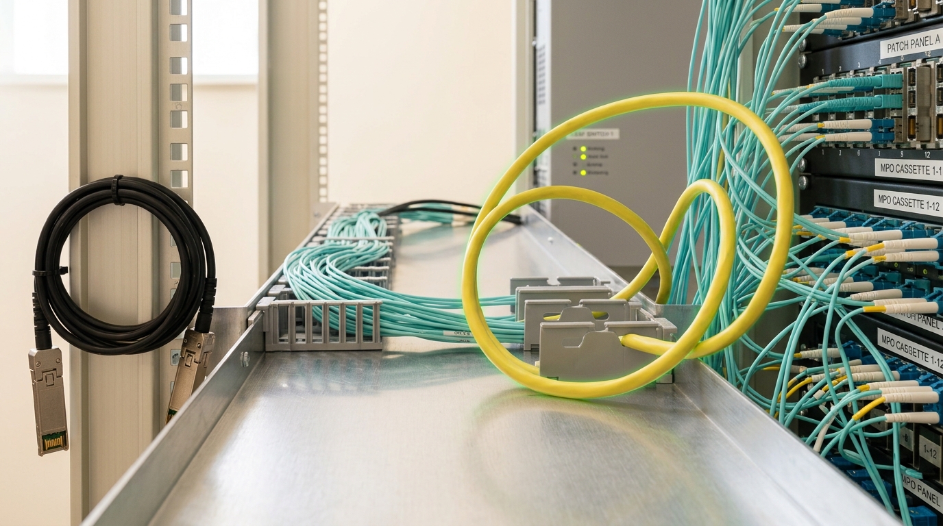
Real systems compose all four, and the composition is where the interconnect asserts itself. The strategies are not interchangeable knobs; each has a characteristic message size, frequency and locality, and a fabric that suits one will strangle another.

What a collective actually costs

The classical accounting for a collective operation separates three terms: a per-message latency, a per-byte transfer cost, and a per-byte computation cost for reductions ^[2]. Writing $\alpha$ for latency per message, $\beta$ for transfer time per byte and $\gamma$ for reduction time per byte, the cost of a collective over $p$ participants on $n$ bytes takes the shape

where $L$ counts message steps, $W$ counts bytes crossing each link and $C$ counts arithmetic. The whole art of collective algorithm design is choosing which of these terms to pay.

Consider the two canonical all-reduce algorithms. A ring arranges participants in a cycle and performs a reduce-scatter followed by an all-gather, each in $p-1$ steps carrying $n/p$ bytes:

The bandwidth term converges to $2n\beta$ as $p$ grows — it stops depending on the number of participants — which is why the ring is the bandwidth-optimal choice for large messages. NVIDIA’s own performance documentation encodes exactly this factor, defining the bus bandwidth of an all-reduce by applying a correction of $2(p-1)/p$ to the naive size-over-time figure, on the reasoning that an all-reduce requires $2(p-1)$ data transfers across $p$ links; all-gather, reduce-scatter and all-to-all get a factor of $(p-1)/p$, while broadcast and reduce get a factor of one because everything must pass through a single root ^[3]. The point of the correction is that bus bandwidth should stay roughly constant as ranks increase, so it can be compared against hardware peak.

But look at the latency term: $2(p-1)\alpha$ grows linearly in the number of participants. A recursive-doubling or tree scheme instead completes in $\lceil \log_2 p \rceil$ rounds:

paying a logarithmic latency term but sending the full message in every round, so its bandwidth cost grows with $\log p$ rather than staying flat.

This is the structural fact underneath everything else in this article: the latency term and the bandwidth term scale in opposite directions with participant count, so no single algorithm is correct. Thakur, Rabenseifner and Gropp’s work on MPICH made the practical consequence explicit — use multiple algorithms per collective depending on message size, minimising latency for short messages and bandwidth for long ones ^[1]. Twenty years later, a modern collectives library is doing the same thing under a different name.

The consequence for model work is direct. Tensor parallelism produces small, frequent messages, so it lives in the latency-dominated regime where $\alpha$ and participant count decide everything. Data parallelism produces one enormous message, so it lives in the bandwidth-dominated regime where $\beta$ decides everything. A fabric optimised for one is not optimised for the other, and a partitioning plan that ignores which regime each of its collectives falls into will be wrong in a way no amount of kernel tuning recovers.

Scale-up and scale-out are different countries

Every large accelerator installation has a boundary in it. Inside a scale-up domain, devices are joined by a dedicated high-bandwidth interconnect; outside it, in the scale-out fabric, they are joined by a datacenter network. The two differ by roughly an order of magnitude in bandwidth and rather more in latency behaviour, and the position of that boundary is the single most important physical fact about the machine.

The magnitude of the gap is well documented by an operator. DeepSeek’s technical report states that in their H800 cluster each node contains eight GPUs joined by NVLink and NVSwitch, with InfiniBand across nodes, and that NVLink offers 160 GB/s of bandwidth, roughly 3.2 times that of InfiniBand at 50 GB/s ^[10]. On the vendor side, NVIDIA claims 900 GB/s per GPU for fourth-generation NVLink, 1,800 GB/s for the fifth generation, and 3,600 GB/s for the sixth, with NVLink Switch aggregate figures rising to 130 TB/s and then 260 TB/s in seventy-two-GPU configurations, and describes sixth-generation NVLink as offering over fourteen times the bandwidth of PCIe Gen6 ^[17]. Those are vendor claims about peak link capability, not measured application throughput, and should be read as such; the relevant point is not the absolute number but the ratio between inside and outside.

That ratio dictates partitioning. Tensor parallelism, with its frequent small collectives in the critical path, belongs strictly inside the scale-up domain. Data parallelism, with its single large periodic all-reduce, tolerates the scale-out fabric. Pipeline parallelism, with its modest point-to-point transfers, tolerates it best of all. Expert parallelism is the awkward case, because all-to-all inherently crosses everything.

DeepSeek’s response to that awkwardness is the clearest illustration in the public literature of a network constraint reaching back into model design. Their report describes a node-limited routing rule ensuring each token is sent to at most a fixed number of nodes — four in their configuration — chosen by affinity scores, so that a token crosses InfiniBand once to reach a node and is then forwarded over the faster in-node NVLink to the specific GPUs holding its experts. They state that twenty streaming multiprocessors suffice to saturate both InfiniBand and NVLink under this scheme ^[10]. The gating function of the model was constrained by the bandwidth ratio of the machine. That is the interconnect writing the architecture.

Different vendors draw the boundary differently. Google’s TPU v4 uses optical circuit switches to reconfigure the interconnect topology dynamically, with the authors reporting that the optical components are under five percent of system cost and under three percent of system power while allowing users to select a twisted three-dimensional torus among topologies across a 4,096-chip system ^[14]. That is a third answer: rather than fixing a scale-up island inside a general fabric, make the topology itself a schedulable resource.

Topology and oversubscription are constraints on the scheduler

Above the scale-up domain, the fabric has a shape, and that shape is rarely uniform.

Meta’s disclosure for Llama 3 is unusually specific. The model was trained on up to 16,000 H100 GPUs within a 24,000-GPU RoCE cluster arranged as a three-layer Clos network, with pods of 3,072 GPUs at full bisection bandwidth but an oversubscription ratio of 1:7 at the aggregation layer above them; the team used a fork of NCCL called NCCLX and applied network-aware job scheduling ^[11]. Read that as a specification of what the scheduler is permitted to do. Below 3,072 GPUs, placement is nearly free. Above it, every collective that spans pods contends for one seventh of the bandwidth it would have had inside one, so the parallelism dimensions must be arranged such that the heaviest and most frequent collectives stay within a pod and only the most tolerant one crosses.

Meta’s network engineering account describes the same structure from the other side: a two-stage Clos “AI Zone” of rack and cluster training switches, with an aggregator layer added to extend the RoCE domain across a building, and cross-zone connectivity oversubscribed by design with traffic balanced using ECMP ^[12]. Alibaba’s HPN paper reports a different bet — a two-tier, dual-plane architecture interconnecting 15,000 GPUs within a single pod, which they note would traditionally require a three-tier Clos, together with a dual top-of-rack design to remove the single point of failure; they report training throughput 14.9 percent higher than a traditional datacenter network and no top-of-rack-related single-node failure over more than eight months in production ^[13]. Wang and colleagues push the argument further, observing that LLM training generates sparse rather than any-to-any communication and proposing a rail-only design that removes the spine layer entirely, which they report reduces network cost by 38 to 77 percent and power by 37 to 75 percent at equal training performance, with an 8.2 to 11.2 percent completion-time overhead for mixture-of-experts all-to-all traffic ^[15].

These are not competing benchmark scores and should not be ranked against one another; they are different design points reached by operators with different workload mixes and different cost structures, and each is reported on its own hardware under its own methodology. What they share is the recognition that the topology is chosen for an assumed communication pattern, which means the scheduler and the parallelism plan are not free variables once the building exists.

A collective runs at the speed of its slowest participant

Bandwidth numbers describe a fabric at rest. Training traffic is not at rest, and its statistical character is unusually hostile to conventional datacenter networking.

Alibaba’s account states that LLM training produces a small number of periodic, bursty flows — on the order of 400 Gb/s on each host — and that this predisposes ECMP to hash polarisation and uneven traffic distribution ^[13]. Meta describes the same phenomenon as low entropy: traffic that is repetitive and predictable, dominated by elephant flows that run at line rate ^[12]. Equal-cost multipath routing was designed for the opposite case — many small independent flows whose hash collisions average out. With a handful of enormous flows, a single unlucky hash collision does not average out; it becomes a persistent hot link.

The reason this matters more for collectives than for ordinary traffic is synchronisation. A collective is a barrier. Every participant waits for the operation to complete, so the operation completes when the last contribution arrives. Tail latency therefore stops being a tail statistic and becomes the mean cost of every step. Dean and Barroso’s analysis of latency variability in large fan-out services is the canonical statement of the mechanism: background activity, queueing at multiple layers including network switches, and shared-resource contention produce occasional slow responses, and a request that must wait on many servers is very likely to encounter one ^[18]. The arithmetic is unforgiving. If each participant independently exceeds its budget with probability $q$, the probability that at least one of $p$ participants does so is

so at a one-percent per-participant rate and 100 participants, roughly 63 percent of collectives are affected — and at 1,000 participants, essentially all of them. That is my own arithmetic on an independence assumption that real systems violate in both directions, but the direction of the effect is not in doubt.

Operators respond by attacking variance rather than mean. Meta reports abandoning DCQCN for its 400G deployments and running with priority flow control alone for over a year, alongside receiver-driven traffic admission in which the collective library coordinates with the RoCE transport to limit in-flight traffic ^[12]. The Ultra Ethernet Consortium’s Specification 1.0, released 11 June 2025 under the Linux Foundation, covers transport, congestion control, direct memory access, link and physical layers and security, and claims end-to-end scalability to millions of endpoints ^[16]. Whether it delivers that in deployed silicon is an open question; it is at present a specification claim.

At this size, something is always broken

The final property of large fabrics is that they are never entirely healthy, and this is a network problem as much as a hardware one because a failed participant halts a collective.

Meta’s Llama 3 disclosure quantifies it. During a 54-day snapshot of pre-training there were 466 job interruptions, of which 419 were unexpected; approximately 78 percent of the unexpected interruptions were attributed to confirmed hardware issues, with GPU-related problems the largest category at 58.7 percent, and the team nonetheless sustained higher than 90 percent effective training time ^[11]. Those are operator-reported figures for one run on one cluster, not an industry rate. But the shape generalises: at tens of thousands of tightly coupled components, mean time between failures for the ensemble falls to hours, and the system design question becomes how cheaply a failure can be detected, isolated and worked around rather than how rarely it occurs.

Network design responds accordingly. Alibaba’s dual top-of-rack scheme exists specifically to remove a single point of failure that would otherwise strand a rack of accelerators ^[13]. Google’s optically switched topology is argued partly on availability grounds, since a reconfigurable interconnect can route around a failed slice rather than losing the machine’s shape ^[14]. And every recovery interacts with placement: replacing a node changes which pod a participant sits in, which changes which collectives cross the oversubscribed layer, which changes step time. Reliability and topology are the same problem viewed from two angles.

What follows in practice

Four rules fall out of the above, and they are the practical content of the argument.

Budget the traffic, not the FLOPs. Before choosing a parallelism plan, write down for each dimension the message size, the frequency, and whether the collective sits in the critical path. That table, not a device datasheet, predicts throughput.

Treat the scale-up boundary as a hard constraint on architecture. Tensor-parallel width should not exceed the high-bandwidth domain, and any routing scheme that produces unconstrained all-to-all across the scale-out fabric should be assumed unaffordable until measured. DeepSeek’s node-limited routing is the template for how to constrain it ^[10].

Measure variance, not just bandwidth. Because collectives synchronise, the useful metric is the distribution of step time, not its mean. A fabric with lower peak bandwidth and tighter tails can beat a faster one.

Assume degraded operation is the normal case. Design the schedule so that a lost node forces a local repair rather than a global re-placement, and report utilisation figures over intervals long enough to include failures.

Predictions, with the observations that would falsify them

These are forecasts, separated from the sourced analysis above. Horizon: 8 August 2029. The assumptions behind all four are that accelerator arithmetic throughput continues to grow faster than per-link electrical bandwidth, and that sparse architectures remain commercially dominant.

One. The scale-up domain will keep growing in accelerator count, and the practical ceiling on tensor-parallel width will rise with it rather than with any change in algorithm. Observable indicator: published high-bandwidth-domain sizes in shipping systems. Disconfirmed if deployed scale-up domains stall at current sizes while tensor-parallel widths grow anyway through algorithmic change.

Two. Routing constraints motivated by network topology — limiting how many nodes a token may reach, or where experts may live — will appear in more published model architectures rather than fewer. Disconfirmed if leading sparse models published in 2029 describe unconstrained global routing and report it as affordable.

Three. Availability rather than bandwidth will dominate published operator accounts: the reported bottleneck in large-run post-mortems will shift from link speed toward failure handling and straggler mitigation. Observable indicator: what large-run retrospectives name as the leading cause of lost throughput. Disconfirmed if those retrospectives continue to attribute lost throughput chiefly to insufficient bisection bandwidth.

Four. Open Ethernet-based transports will take meaningful share of scale-out fabrics while proprietary interconnects retain the scale-up domain. Disconfirmed if a single vendor’s fabric spans both tiers in the majority of new large deployments, or if Ethernet displaces the proprietary scale-up interconnect as well.

None of these requires a technological discontinuity. They follow from the cost structure already visible: two terms that scale in opposite directions, a hard bandwidth boundary inside every machine, and a failure rate that rises with the component count.

What to take away

A model spread across devices is a communication schedule first and an arithmetic workload second. Each parallelism strategy generates a distinct traffic pattern — one large periodic reduction, many small critical-path collectives, sparse point-to-point transfers with idleness attached, or a data-dependent scatter that touches everything. Each of those patterns falls in a different regime of a cost model whose latency term and bandwidth term move in opposite directions as participants are added, which is why no single collective algorithm and no single fabric is correct.

Around that sits a machine with a hard internal boundary, a topology chosen for an assumed pattern, an oversubscribed layer that turns placement into a first-class scheduling constraint, a traffic distribution that defeats the load-balancing assumptions of ordinary datacenter networking, and a component count high enough that something is always broken. Every one of those is a reach problem, not a speed problem. The relays in a repeater station were never there to make the signal faster.