Say “domestication began around 10,500 years ago in the Fertile Crescent” and it sounds like a date on a calendar. It is not. It is the output of a specific inference chain — mandible wear stages tallied into a mortality curve, a handful of enamel samples drilled and run through a mass spectrometer, a genome assembled from a few hundred thousand damaged DNA fragments — and every link in that chain has a documented error bar. This guide walks through the methods themselves: how a zooarchaeologist decides an animal population was managed rather than hunted, how an ancient-DNA lab pulls a usable genome out of a burnt seed, and how a survey team turns a scatter of potsherds into a population estimate for a settlement whose walls no longer stand. The point is not to undermine the big picture — cereal and animal domestication, urbanization, and state formation are not in serious dispute — but to show what actually stands underneath the round numbers, and where that support gets thin.
1. What “domesticated” means operationally, and how you test for it
Domestication is not a single moment; it is a shift in a population’s demographic and morphological profile produced by sustained human management, and it has to be inferred from indirect proxies because nobody recorded the transition in writing. Three independent proxies are used, and the practice in a rigorous zooarchaeological report is to require agreement across at least two before calling a faunal assemblage “managed” rather than “hunted.”
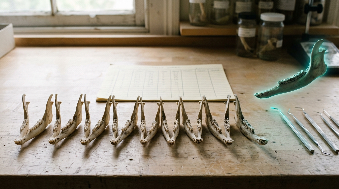
Kill-off (age-at-death) profiles. Sebastian Payne’s 1973 study of sheep and goat mandibles from Aşvan Kale set the still-standard method: use tooth eruption and wear stages to sort a mandible assemblage into age classes, then compare the resulting mortality curve against three idealized target profiles — one that maximizes meat yield (heavy juvenile culling), one that maximizes milk (very young males culled, females kept to breeding age), and one that maximizes wool (both sexes kept well into adulthood) [3]. A wild hunted population’s age structure tracks natural mortality; a managed herd’s age structure tracks whichever product the herders were optimizing for. The method is entirely about shape of the curve, not presence or absence of an animal — this is the part that gets flattened in popular summaries. Fact: this is the method Payne published and it remains the reference point cited in current mortality-profile studies. Analysis: the method assumes the three idealized profiles are exhaustive and that a mixed-strategy herd (real herds rarely optimize for only one output) will show up as a blend rather than a fourth category — a real limitation acknowledged in the method’s own literature, not a flaw specific to any one site.
Bone morphology and size reduction. Domestic populations of cattle, sheep, goat, and pig consistently run smaller than their wild progenitors within a few centuries of initial management, a phenotypic response to selection and constrained diet. Measurement of long-bone dimensions against wild reference populations is a standard supporting line of evidence, though it lags kill-off evidence in onset — size reduction shows up after management has already begun, so its absence in an early assemblage does not rule out domestication in progress.
Isotope-based weaning and seasonality reconstruction. This is the proxy that actually distinguishes “wild population culled by humans” from “population whose reproduction and diet humans were controlling.” A tooth’s enamel forms sequentially, layer by layer, over the animal’s early life, so drilling a sequence of small samples along the tooth’s growth axis and running each through an isotope-ratio mass spectrometer for δ13C and δ15N (and δ18O for season-of-birth) recovers a month-by-month record locked into a single tooth [4]. Nitrogen isotopes are the weaning signal specifically: a nursing juvenile sits roughly one trophic level above its mother, a 3–3.5‰ δ15N offset that collapses once weaning is complete. An abrupt, human-timed weaning point — rather than the gradual, food-availability-driven weaning of a wild population — is direct evidence of herd management, because someone decided when the milk stopped, not the animal. Sequential enamel work on Tell Halula cattle applied exactly this design to Syrian Neolithic material and recovered management-consistent weaning timing distinct from wild seasonal patterns [9]. Fact: the trophic-offset magnitude and the sequential-sampling method are established and widely replicated. Analysis: a single molar gives you one individual’s early-life record; a defensible claim about herd-level practice requires sampling enough individuals to see a consistent pattern, not one anomalous tooth, and published studies vary considerably in how many individuals they sample per site — a genuine source of disagreement between papers on the same site.
Put together, a domestication claim for a given site and period should cite: a kill-off profile skewed toward one of Payne’s target shapes, isotope evidence of controlled weaning timing, and ideally a size trend — not any one of these alone. Reviews of Neolithic Southwest Asian cattle management explicitly triangulate demographic (kill-off), morphometric (size), and isotopic evidence for exactly this reason [10].
2. Getting a genome out of a burnt seed or a buried bone
Ancient DNA (aDNA) work on domesticates answers a different question than zooarchaeology: not “was this population managed” but “where did the founding population come from, and how did later gene flow reshape it.” The methodology has changed almost completely twice since the 1980s, and it is worth being specific about which generation of results you are reading.
Phase one (1980s–2000s): PCR amplification of mitochondrial DNA. Early work targeted the mitochondrial control region because mtDNA exists in thousands of copies per cell versus one or two for nuclear DNA, making it far more likely to survive degradation. This phase established that modern livestock descend from multiple, geographically distinct wild progenitor lineages rather than a single domestication event — an important finding — but mtDNA is maternally inherited only, so it is blind to male-line history and to admixture from a second domestication center [1].
Phase two (post-2005): high-throughput shotgun sequencing. Massively parallel sequencing-by-synthesis, built for exactly the short, damaged fragments ancient bone yields, cut sequencing cost by roughly five orders of magnitude between 2007 and 2019, and made whole-genome (not just mitochondrial) ancient sequencing routine [1].
Phase three (post-2014): petrous-bone targeting. A single methodological discovery reset sample strategy across the field: the petrous portion of the temporal bone, the densest bone in the mammalian skeleton, yields dramatically higher fractions of endogenous (non-contaminant) DNA than any other skeletal element routinely available from an excavation. Labs now prioritize petrous samples and dental cementum over the long bones and ribs that early aDNA studies had to rely on [1].
The wet-lab pipeline in practice, condensed to its decision points:
- Sampling in a dedicated clean room, physically separated from any modern-DNA lab in the same building, positive-pressure, full protective clothing, UV-irradiated surfaces — because a single modern skin-cell contaminant can outcompete a degraded ancient template during amplification.
- Milling a small quantity of bone or dentine to powder, then chemical extraction (typically a silica-column or magnetic-bead binding step) that is tuned to retain the very short (often 40–80 base pair) fragments characteristic of degraded DNA, since standard modern-DNA extraction kits are optimized for longer fragments and lose most of the ancient signal.
- Library preparation with damage-aware adapters, since ancient DNA carries a signature pattern of cytosine-to-thymine misincorporation concentrated at fragment ends from post-mortem deamination — a pattern labs now use positively, as a built-in authentication check that distinguishes genuinely ancient reads from modern contamination.
- Shotgun or targeted-capture sequencing, followed by bioinformatic alignment to a reference genome and read-depth and damage-pattern filtering before any population-genetic inference is drawn.
Fact: every step above is documented lab practice in the aDNA literature, not vendor description. Vendor-claim flag: sequencing-instrument manufacturers routinely advertise “ancient-DNA-optimized” kits and workflows; those marketing claims are not independently substituted for the peer-reviewed damage-pattern authentication step above, which remains the actual community standard regardless of which vendor’s reagents were used.
Charred crop seeds present a harder case than bone: charring can both preserve and further degrade DNA depending on temperature and duration, and contamination risk from modern airborne plant material is higher in the field than for buried bone. Plant aDNA studies accordingly report lower success rates and shorter average fragment recovery than comparable animal-bone studies — a methodological asymmetry worth noting whenever a crop-domestication genetic claim is compared directly against a livestock one.


3. From potsherds to population: settlement-pattern survey arithmetic
Ask how large an ancient city was and you will usually get a single confident number. The number is downstream of a specific, contestable arithmetic: estimated population = settled area × occupational density, where “occupational density” (people per hectare) is not measured directly but assumed from ethnographic analogy or from settlements where structural remains happen to survive well enough to count houses.
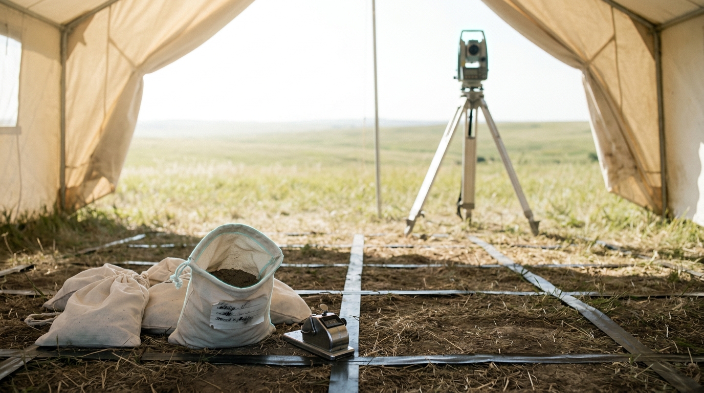
Pedestrian survey is the field method that produces the area estimate: a team walks a predetermined grid or transect across a landscape, systematically collecting or tallying surface artifacts (sherds, lithics, tile) into gridded bags per unit of ground, and plots artifact density against location to define a site’s boundary and internal density gradient rather than relying on visible mounding alone. The area figure that later gets multiplied by a density constant comes directly out of this artifact-density mapping.
The catch, documented directly in the settlement-archaeology literature, is that occupational density is not a fixed constant — it varies by region, period, and settlement size, and the relationship between the two is itself an empirical question rather than a known input [8]. Studies applying settlement-scaling theory — originally developed for modern cities, where built area and population follow measurable statistical regularities — to pre-Hispanic Mesoamerican settlement systems (the Basin of Mexico survey record) found that ancient settlement area and estimated population obeyed a scaling relationship with an exponent in roughly the 2/3 to 5/6 range, structurally similar to modern urban scaling laws despite radically different technology and political organization [5]. That is a real, quantitative, falsifiable finding about how area and population relate — but note what it does not do: it does not independently verify the absolute population number for any one site, because the underlying density constant used to calibrate the model is still drawn from the same ethnographic-analogy or partial-excavation sources as any other method. Two honest population estimates for the same Bronze Age city, built by different survey teams using different density assumptions, can and do disagree by a factor of two or more, and any single-figure population claim you read for a prehistoric city should be treated as the midpoint of that kind of range, not a census result.
Scenario, clearly flagged as such: if lidar-based subsurface mapping and multispectral crop-mark detection continue to cut the cost of full-coverage survey (an ongoing, observable trend rather than a settled fact), occupational-density estimates for well-surveyed regions could shift from ethnographic analogy toward direct structure counts within the next one to two decades. Horizon: 2035–2045. Assumption: continued public and grant funding for remote-sensing survey campaigns. Observable indicator: a measurable rise in structure-count-based (rather than analogy-based) density figures in published survey reports for a given region. Disconfirmation condition: if remote-sensing-derived structure counts, once available at scale, converge closely with existing ethnographic-analogy density figures, that would show the analogy approach was already tracking reality reasonably well, undercutting the case that a methodological shift changes the resulting numbers much.
4. Disease, density, and the epidemiological cost of settling down
Sustained proximity to livestock and to other humans at higher density than foraging bands sustained is a mechanism, not an assumption, for the rise of new human infectious disease after the adoption of agriculture. A widely cited review identifies five stages through which a pathogen exclusively infecting animals can become a pathogen exclusively infecting humans, moving from occasional spillover with no onward human transmission through to a fully human-adapted disease that no longer needs the animal reservoir at all, and finds that the great majority of documented major human infectious diseases are evolutionarily recent, arising only after agricultural origins, and overwhelmingly of Old World rather than New World origin [7]. That asymmetry — Old World disease burden dramatically exceeding New World — tracks the asymmetry in domesticated animal species available on each continent, itself a consequence of which wild progenitor species existed there to begin with, not a claim about the peoples themselves.
Analysis, not fact: it is tempting to read this as “agriculture caused disease,” full stop, but the mechanism is more specific and more contingent: it required domesticated animal species living in close, sustained contact with humans, at settlement densities sufficient to sustain person-to-person transmission chains once a pathogen made the jump. Regions that adopted intensive plant agriculture without comparable livestock density (parts of the pre-contact Americas, for example) did not see the same disease burden, which is evidence for the animal-contact mechanism specifically rather than agriculture or density alone.
5. Reading a collapse: what a paleoclimate proxy can and cannot tell you
Claims that a specific ancient state collapsed “because of” an abrupt climate event are among the most overstated in popular treatments of this material, and the methodology is worth separating from the conclusion. The reference case is the Akkadian-era collapse in northern Mesopotamia: excavation and soil-stratigraphic work at Tell Leilan documented a marked increase in aridity and wind-blown sediment beginning around 2200 BCE, following a period of urban growth on the Habur Plains, with regional abandonment following the onset of that aridity shift and roughly synchronous disruption reported in the Aegean, Egypt, and the Indus [6].
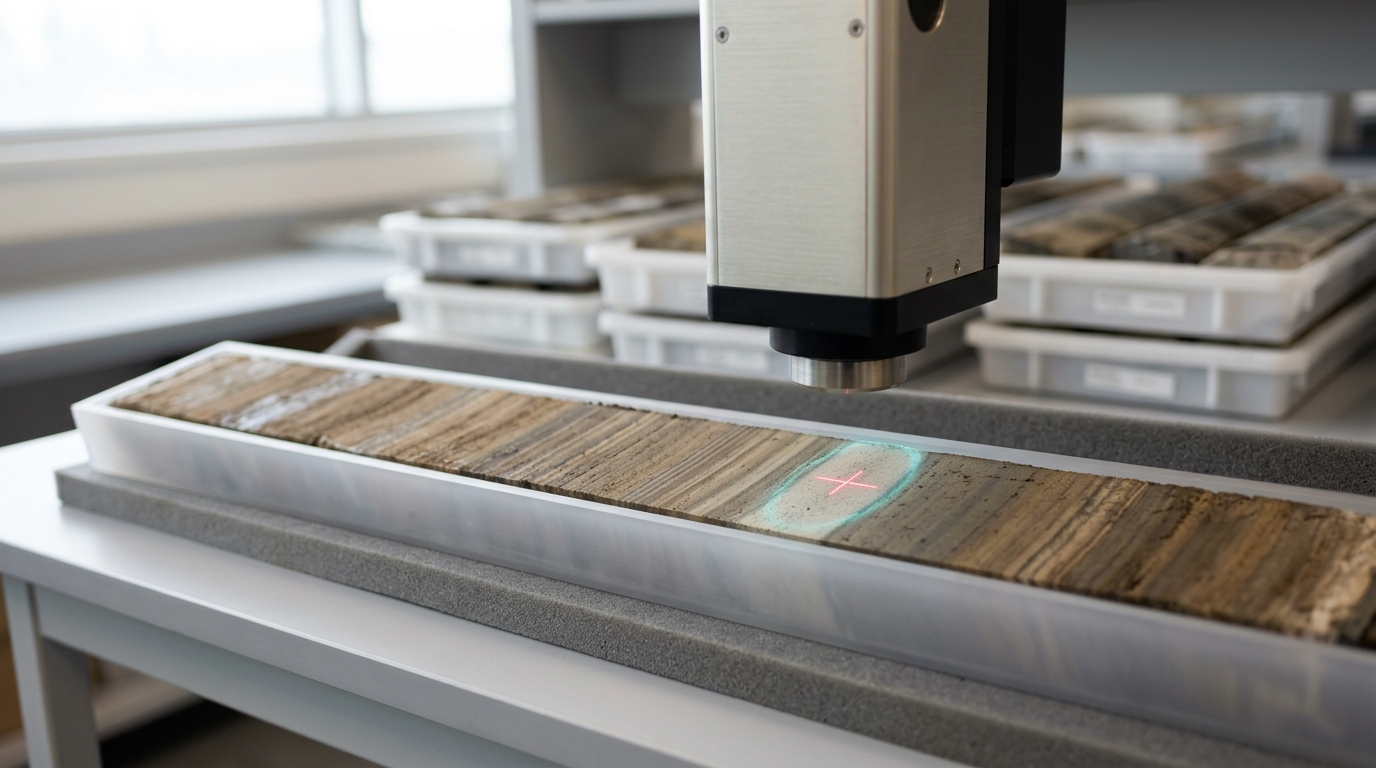
The evidentiary chain here has a specific structure worth naming: (1) a paleoclimate proxy — here, wind-transported sediment and soil geochemistry, elsewhere annually laminated lake or cave records — establishes that an abrupt environmental shift occurred at a datable horizon; (2) an archaeological abandonment signal — occupation debris ending, structural collapse layers, survey-detected settlement desertion — establishes that human occupation changed at a broadly compatible horizon; (3) correlation in time is not, by itself, causal attribution. The original 1993 study was explicit that synchronous disruption across separate regions strengthens the case for a shared climatic trigger over a series of independent local political failures that happened to coincide, but a single-region case built on proxy dating alone cannot rule out a political or economic account, or a compound explanation in which climate stress interacted with pre-existing administrative strain rather than causing collapse on its own. Later scholarship on this specific event has continued to debate the relative dating precision between the climate proxy and the archaeological abandonment horizon — a genuine, unresolved disagreement in the literature, not a settled consensus that this guide should paper over.
6. Regional diversity: why one method set does not travel everywhere
Every method above was developed, validated, and most heavily applied in a specific region — Southwest Asian zooarchaeology for kill-off profiles, European and Southwest Asian faunal assemblages for weaning isotopes, Mesoamerican survey data for settlement scaling, Near Eastern sediment sequences for the collapse case. Applying any one of them elsewhere requires re-validating its assumptions against local conditions, not importing the numbers directly.
Kill-off profile targets calibrated for sheep and goat husbandry do not transfer cleanly to cattle, whose reproductive biology and product mix (traction, milk, meat) differ enough that Payne’s three idealized curves need re-derivation rather than direct reuse — work that has been done for cattle specifically but is a separate literature from the original caprine study. Settlement-scaling exponents derived from the Basin of Mexico survey record are an empirical finding about that particular settlement system’s growth dynamics; the original paper itself frames the result as a theory to be tested against other regions’ survey data, not a universal constant already established for all pre-modern urbanism [5]. And the isotope-based weaning method depends on a species- and region-specific baseline for the pre-weaning trophic offset, which has to be established locally (often via modern reference animals raised under known conditions) before it can be applied to an archaeological assemblage with confidence [4].
Prediction, explicitly scoped: as regional aDNA and isotope reference datasets for South Asia, East Asia, and sub-Saharan Africa continue to be built out — currently thinner than the Southwest Asian and European record — expect the geographic center of gravity for domestication and early-urbanism method papers to shift measurably away from the Fertile-Crescent-and-Mesoamerica focus of the last three decades. Horizon: 2030–2040. Assumption: continued funding for aDNA infrastructure outside its current concentration in European and North American labs. Observable indicator: a rising share of major domestication and settlement-density papers using primary non-Fertile-Crescent, non-Mesoamerican datasets. Disconfirmation condition: if funding and lab-infrastructure growth remains concentrated in already-established regions, the current geographic imbalance in the literature will persist rather than close.
Method summary: what each claim actually rests on
| Claim type | Primary method | What it directly measures | What it does not establish alone |
|---|---|---|---|
| “This population was domesticated” | Kill-off profile (tooth wear/eruption) | Age-at-death distribution shape | Which product was prioritized, without isotope corroboration |
| “Weaning was human-controlled” | Sequential enamel isotopes (δ13C, δ15N) | Trophic-level shift timing in one individual | Herd-wide practice, without multiple individuals sampled |
| “This lineage’s ancestry traces to X” | Ancient DNA (shotgun/capture sequencing) | Genetic similarity and admixture proportions | Where domestication behaviourally began, independent of genetics |
| “This city held N people” | Pedestrian survey + area-density model | Settled area and artifact density | Absolute population, without an independently validated density constant |
| “Climate caused this collapse” | Paleoclimate proxy + abandonment horizon | Temporal correlation of two datable events | Causal mechanism, without a documented pathway connecting them |
None of this weakens the broad synthesis — that agriculture, cities, hierarchy, and disease burden are causally entangled processes visible across many independent regional records. It is a case for reading population figures, domestication dates, and collapse narratives as inference chains with named, checkable steps, each of which can in principle be wrong in a specific, falsifiable way, and none of which should be quoted as a bare number without knowing which step it actually rests on.
Sources rejected during verification
One candidate source — a Nature-hosted article behind an institutional sign-in wall that could not be confirmed as openly accessible — was dropped in favor of the equivalent open PMC-hosted reprint and the BMC Biology paleogenomics review already cited, which cover the same methodological ground and were directly verifiable.