What Interpretability Actually Costs to Do at Scale

Two ledgers, not one

Public arguments about mechanistic interpretability are almost always arguments about whether the method works — whether a recovered feature is real, whether a circuit explanation is faithful, whether a dictionary has found the model’s own units or invented a convenient fiction. Those are the right questions, and this publication has asked them at length elsewhere ^[2]. They are also, on their own, incomplete, because a research programme does not run on being right. It runs on a budget, and interpretability has two of them that are frequently collapsed into one.

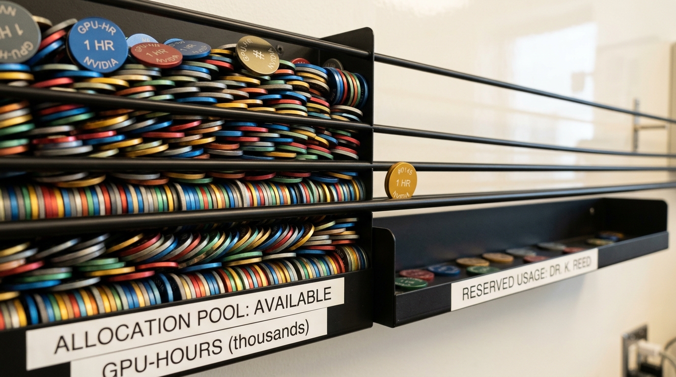
The first is a compute ledger: the GPU-hours spent training a sparse dictionary on a frontier model’s activations, and the GPU-hours spent afterward running interventions against it. The second is a labor ledger: the analyst-hours spent turning a statistically clean result into a claim that has actually met a faithfulness standard — not “this direction correlates with the concept” but “we changed this and the model’s behavior changed in the way the story predicts, robustly, across the alternative explanations someone competent would raise.” These two ledgers are paid in different currencies, by different people, on different timescales, and conflating them is how a research area ends up simultaneously described as “the compute is basically free, it’s a rounding error on the training run” and “understanding one behavior took a team-month,” both said by people who are right about their half of the ledger.

This article works through both ledgers in turn, with numbers, then asks the only question that actually matters for whether the field can keep up with what it is trying to interpret: does either cost fall as models get bigger, or does it rise, and by how much.

What a sparse autoencoder actually costs to train

Start with the compute side, because it has the one number in this literature precise enough to build an equation around.

A sparse autoencoder (SAE) is trained to reconstruct a model’s internal activation vectors through a sparse bottleneck: an encoder maps an activation of dimension $d$ into a much wider space of $n$ candidate “features,” a sparsity constraint keeps only $k$ of those features active per token, and a decoder reconstructs the original activation from just those $k$. The training objective, in its standard form, is

and the specific variant OpenAI’s interpretability team used to push this to frontier scale, the TopK autoencoder, replaces the soft $\ell_1$ penalty with an explicit constraint: exactly $k$ latents fire, chosen by magnitude, and the rest are hard-zeroed. Gao and colleagues introduced this variant, established scaling laws relating autoencoder size and sparsity to reconstruction error, and — this is the operative fact for a cost accounting — trained a sixteen-million-latent autoencoder on GPT-4’s activations over forty billion tokens ^[1].

Work out what that architecture actually spends compute on per token, because the two halves of it behave differently. The encoding step needs a score for every one of the $n$ candidate latents before it can select the top $k$, so it is an unavoidably dense matrix multiply: roughly $2dn$ floating-point operations. The decoding step only touches the $k$ latents that survived, so it is sparse: roughly $2dk$ operations. Summed and multiplied across $T$ training tokens, a first-order compute model for training the dictionary is

Because published TopK configurations keep $k$ in the tens to low hundreds while $n$ runs into the millions, $n \gg k$ and the encoding term dominates almost entirely: $C_{\mathrm{SAE}} \approx 2dnT$. That single approximation explains something the paper reports without deriving: convergence — the point at which more tokens stop buying lower reconstruction error — is reached later as $n$ grows, empirically as $\Theta(n^{0.65})$ tokens for GPT-4-scale autoencoders ^[1]. Cost scales with the product of dictionary width and token count, and pushing width up forces token count up too if the dictionary is to be trained to convergence rather than merely trained. The paper is explicit that this collided with a real constraint: at their largest scale they state plainly that “because of compute constraints, we were unable to train our 16 million latent autoencoder to” the convergence frontier they used for smaller runs ^[1]. Sharkey and colleagues, surveying the field’s open problems, draw the economic conclusion directly: sparse dictionary learning “will probably be relatively expensive to train compared to the original model” it is being used to interpret, and that expense compounds because a separate dictionary is typically needed for every layer an investigator wants to see into ^[2].

The one number that pins this down, and what it is not

Gao and colleagues report a figure that is, as far as this article’s research turned up, the clearest published tie between SAE cost and a frontier model’s own training budget: “when our 16 million latent autoencoder is substituted into GPT-4, we get a language modeling loss corresponding to 10% of the pretraining compute of GPT-4” ^[1]. Read carelessly, that sentence sounds like a FLOP count — as though the dictionary’s training run burned an amount of compute equal to a tenth of GPT-4’s own pretraining. It is not that. It is a capability-equivalent cost: patch the dictionary’s reconstruction into the model in place of the true activations, measure how much the model’s own performance degrades, and ask how much pretraining compute would have to be removed to produce a model that bad by itself. The answer is: a lot. Ninety percent of GPT-4’s pretraining compute, thrown away, would degrade the model to roughly where the reconstruction error from the largest published dictionary already leaves it.

This distinction matters for the argument of this article, not just for precision’s sake. Two different quantities are both real costs, and they point in the same direction for different reasons. The training-compute cost — tokens times dictionary width, from the equation above — is a bill the lab pays once, upfront, in GPU-hours, and it is large enough that OpenAI’s own paper reports hitting a compute ceiling before reaching the same convergence standard used at smaller scale. The reconstruction-fidelity cost — the 10% figure — is a bill paid every time the dictionary is actually used as a stand-in for the model’s true internals, because an imperfect reconstruction is imperfect exactly where a downstream mechanistic claim would need it to be exact. A dictionary can be expensive to build and still not be trustworthy to lean on, and both of those are cost problems, not the same cost problem.

Anthropic’s parallel effort, training sparse autoencoders with up to thirty-four million features on Claude 3 Sonnet’s middle-layer residual stream, reached comparable scale and reported the same character of shortfall from the inside: “our suite of features is incomplete, and we lack rigorous methods for evaluating whether our features faithfully capture model computations” ^[3]. A laboratory that had just spent enough compute to train a thirty-four-million-latent dictionary on its own flagship model, and whose own paper concedes incompleteness in the next sentence, is not being modest. It is reporting that the compute ledger and the trustworthiness ledger do not close against each other automatically — spending more on the first does not guarantee anything about the second.

Verifying a circuit is a different kind of expense

Move to the labor side, where the accounting is harder because almost nobody publishes it. Papers report ablation counts and head counts; they very rarely report the thing a cost model actually needs, which is researcher-hours.

One paper does, because measuring exactly that was its purpose. Marks and colleagues ran a blind auditing game: a model was deliberately trained with a concealed objective, and four teams — with varying levels of access, from full training-data visibility to API-only — were set loose to find it, with their working time logged ^[4]. The published table is the closest thing this literature has to a labor-cost line item: one team surfaced the hidden objective in 1.5 total researcher-hours; a second took 11 serial hours and 31 cumulative researcher-hours across its members; a third took 6 serial hours and 10 cumulative hours; the fourth team, restricted to black-box API access with no interpretability tooling, logged more than 70 cumulative researcher-hours and still did not succeed ^[4]. Three of the four teams that succeeded had privileged access — to weights, activations, or training data — and the paper’s own honest caveat is that team composition varied enough that the numbers cannot be read as a clean method comparison. But as an order of magnitude for what “verify one specific claim about a specific model” costs in human time, even under favorable, cooperative conditions with a known ground truth waiting to be found, the answer sits somewhere between a long lunch and two working weeks.

Contrast that with what it took to fully triangulate a single mechanism to the field’s own satisfaction rather than to win a game with a known answer. Olsson and colleagues’ induction-head result — the most thoroughly evidenced mechanistic claim in the published literature — rests on “34 transformers over the course of training, including more than 50,000 attention head ablations” ^[7], assembled into six independent lines of evidence: a training phase change, architectural manipulations that shift it, direct ablation, generality across behaviors, generalization from small models, and continuity to larger ones. That is not the cost of finding a candidate mechanism. It is the cost of ruling out the ways the candidate could have been an illusion — a different, and much larger, expenditure. The indirect object identification circuit in GPT-2 small tells the same story from a different angle: twenty-six attention heads sorted into seven functional classes, found through causal intervention and checked against three explicit criteria the authors had to define from scratch — faithfulness, completeness, and minimality — because before that paper “we found a circuit” carried no falsification condition at all ^[8]. Both papers describe themselves, without irony, as the most extensive attempt of their kind to date. Both are analyses of one behavior, in one small model.

A simple model makes the scaling problem legible. Let a verified circuit claim require passing $m$ distinct checks — faithfulness under intervention, completeness against the behavior it is meant to fully explain, minimality against components that turn out not to matter — and let each check take $h_i$ researcher-hours, including the false starts a competent skeptic would force. Total verification cost per claim is

and the field’s own most careful examples put each $h_i$ measured not in minutes but in dedicated researcher-days once ambiguity has to be resolved rather than merely observed. If a frontier model implements even a low four-figure count of distinguishable, individually claim-worthy behaviors — a conservative floor, not an estimate anyone has actually published, because nobody has enumerated a frontier model’s behavior inventory any more than its feature inventory — then $H_{\mathrm{verify}}$ summed across even a small fraction of them outruns any realistic standing research team within a single model generation, let alone across the several generations a lab now ships per year. This is precisely the bottleneck the field’s own methods papers name as the reason automation is not optional: Conmy and colleagues built an algorithm to prune the computational graph automatically because, in their words, “the current approach to extracting circuits from neural networks relies on a lot of manual inspection by humans,” which is “a major obstacle to scaling up mechanistic interpretability to larger models, more behaviors, and complicated behaviors composed of many sub-circuits” ^[9]. Their validation of that automation was itself modest by design — recovering, on GPT-2 small, five component types and sixty-eight of thirty-two thousand edges that had already been found by hand in prior work ^[9]. Recovering a known answer faster is real progress on the labor ledger. It is not evidence that automation finds what a human would have missed.

The most advanced automated attempt, and its own coverage numbers

The most technically ambitious published answer to the labor problem is Anthropic’s attribution-graph method, which builds a “replacement model” out of cross-layer transcoder features and constructs a computational graph automatically rather than by hand-driven activation patching ^[5]. It is worth reading its own accounting of what automation currently buys, because the authors report it with unusual candor.

The replacement model’s fidelity is bounded: their largest configuration “matches the underlying model’s next-token completion on 50% of a diverse set of pretraining-style prompts” ^[5] — a coin flip, on prompts not chosen to be adversarial. Where it does produce a graph, the companion paper applying the method to real behaviors in Claude 3.5 Haiku reports that the resulting attribution graphs give “satisfying insight for about a quarter of the prompts we’ve tried” ^[6], and both papers are explicit that even a successful graph explains only part of the computation: perturbation experiments track the underlying model’s actual behavior at roughly 0.8 cosine similarity one layer downstream of an intervention, degrading further with distance ^[5], and the method has a structural blind spot — it does not explain how attention patterns themselves form, so “we have also found many cases where this limitation renders our attribution graphs essentially useless” ^[5]. Building the replacement model in the first place is described as carrying “significant up-front cost and effort, which is amortized over its application to circuit discovery” ^[5] — automation here is a large fixed capital cost traded against a smaller, but still nonzero, marginal cost per behavior investigated, not a route to zero marginal cost.

Put the coverage numbers next to each other and a specific shape appears, not a vague one: a fixed up-front compute cost buys a tool that works, by the authors’ own count, on roughly a quarter of what it is pointed at, matches ground truth on about half of ordinary prompts even where it does produce output, and is honestly flagged as sometimes useless for an entire class of mechanism. That is real progress against the manual-inspection baseline. It is also, on the numbers its own authors published, nowhere near a solved coverage problem.

The historical resourcing gap

None of the above would matter much if interpretability’s budget — either ledger — had simply kept pace with the systems it studies. The documented record says it has not, and the clearest evidence is a promise that was made and then not kept.

In July 2023, OpenAI announced its Superalignment effort with a specific, checkable commitment: 20% of the compute the company had secured to date, dedicated to the problem over four years. Reporting based on six sources familiar with the team’s operation found the commitment was never honored — the team’s compute budget “never came close to the promised 20% threshold,” requests for additional GPU access “were routinely rejected by higher-ups,” and the team’s co-lead wrote internally that “my team has been sailing against the wind. Sometimes we were struggling for compute and it was getting harder and harder to get this crucial research done” before the team was dissolved ^[10]. Whatever the ambiguity in how “20%” was meant to be measured — annualized, front-loaded, cumulative — the gap between a public commitment and an internal budget fight is not ambiguous, and it is the single most concrete data point available on how a frontier lab actually prioritizes interpretability-adjacent compute against its own production and pretraining demands when the two compete for the same cluster.

The pattern is not confined to one company’s internal budget fight. Independent field-level accounting from the 2025 State of AI Report puts a number on the disparity between capability-side and safety-side resourcing across the whole external ecosystem: “all 11 major US safety orgs will spend $133M in 2025 — less than frontier labs burn in a day” ^[11]. That figure is about safety research broadly, not interpretability narrowly, and interpretability is only one line inside it — but it is the best available anchor for the relative scale of the two research programmes, capability and oversight, that this article’s opening ledger split apart. A policy memo from the Federation of American Scientists frames the resulting timeline mismatch directly: AI companies’ own projections put reliably understanding model internals at five to ten years out, against expert expectations of human-level general-purpose capability arriving as soon as 2027 ^[13]. Whether or not that capability timeline proves accurate — this article takes no position on it — the structural point survives either way: the resourcing and the research horizon of interpretability were set, historically, as though the systems under study would hold still long enough to be caught up with.

There is a countervailing data point, and it is recent enough that it changes the shape of the argument rather than just adding a footnote to it. Interpretability has begun attracting substantial private capital as a product category in its own right, separate from any lab’s internal safety budget: Goodfire, an AI lab built specifically around interpretability, raised a $150 million Series B in February 2026 at a $1.25 billion valuation, explicitly to “enhance its platform and finance AI interoperability research projects” ^[12]. That is a real, large, freshly committed sum, and it did not exist as a funding category running through venture capital even two years earlier. It is also a fundamentally different kind of money from a lab’s internal compute allocation: it is capital betting that interpretability-as-a-service is a viable commercial product, not a lab committing its own training cluster to auditing its own frontier model. Both are real resourcing. They are not substitutes for each other, and conflating “interpretability is attracting money” with “interpretability is getting the compute allocation inside the labs that most need auditing” would be exactly the kind of ledger-collapsing this article opened by warning against.

Does the interpretability tax scale

Put the two ledgers and the resourcing record together and the honest answer to “can interpretability scale to audit systems as they grow” is: not on the current trajectory of either cost, and the reasons differ by ledger.

The compute ledger has a plausible, if unproven, path downward. $C_{\mathrm{SAE}} \approx 2dnT$ is a cost that infrastructure and algorithmic improvements — sparser encoders, better initialization that reaches convergence at lower $n$, transcoders that replace rather than merely observe a component — can attack directly, the same way serving-side engineering rather than raw parameter growth has driven most within-generation price reduction for inference elsewhere in this field. TopK autoencoders were themselves exactly this kind of improvement over the softer, less efficient sparsity penalties they replaced ^[1]. There is no comparable engineering lever visible yet for the labor ledger. $H_{\mathrm{verify}}$ is bounded below by the number of independent lines of evidence a claim needs before it stops being a good story and starts being a checked fact, and every fully triangulated example this field has published — induction heads, indirect object identification — got there by adding more human-driven checks, not fewer. Automated circuit discovery and attribution graphs are real progress against that floor, but on their own authors’ published numbers they currently trade a large fixed compute cost for partial coverage — a quarter of prompts yielding satisfying insight, half of ordinary completions matched, whole mechanism classes still out of reach — rather than for full replacement of the manual check ^{[5, 6]}.

That asymmetry is the actual content of “the interpretability tax.” It is not one tax; it is two, falling on different budgets, and only one of them behaves like an engineering problem that better hardware and better algorithms predictably shrink. The other behaves like an evidentiary standard, and evidentiary standards do not get cheaper just because the thing being investigated got bigger — if anything, a larger, more capable model plausibly has more distinguishable behaviors worth an audited claim, which pushes total verification cost up even if the per-claim cost held flat. Nobody has published a credible estimate of how many claim-worthy behaviors a frontier model actually contains, which is itself a symptom rather than an incidental gap: a field cannot cost its own labor budget against a behavior inventory it has not built.

Predictions, with what would falsify them

These are forecasts, clearly separated from the sourced analysis above. Horizon: August 2029. Assumptions: no change in the dominant transformer architecture, continued publication norms at the major interpretability groups, and no regulatory mandate forcing a specific interpretability standard before deployment.

One. Published per-token or per-latent SAE training cost will fall faster than published verification-hours-per-claim, because the first is an engineering target with clear proxy metrics (reconstruction MSE, dead-latent rate) and the second is not. Disconfirmed if a published method cuts researcher-hours-to-verified-claim by an order of magnitude without a corresponding, comparably documented drop in what counts as “verified.”

Two. Labs will increasingly report automated-method coverage statistics of the kind Ameisen and colleagues published — fraction of prompts matched, fraction yielding satisfying insight — as a standard disclosure, because the alternative, reporting only successful case studies, will have become recognizably unfalsifiable in a crowded field. Disconfirmed if 2029’s leading interpretability papers still report case studies with no denominator.

Three. Private interpretability-focused capital (Goodfire and its category peers) will grow faster than internal lab compute commitments to interpretability, widening rather than closing the gap between “interpretability the product” and “interpretability the safety function inside the lab building the frontier model.” Disconfirmed if a frontier lab publishes and independently verifiable, honored compute-share commitment to interpretability of the kind promised and not delivered in 2023.

Four. No published audit of a frontier system by 2029 will rest primarily on mechanistic evidence with a stated, met completeness bar; behavioral and black-box evaluation will remain the load-bearing evidence in practice, with mechanistic findings as corroboration. Disconfirmed if a third-party audit of a frontier model is published that certifies the absence of a specific property primarily on circuit-level evidence meeting explicit faithfulness, completeness, and minimality criteria.

What to take away

Interpretability’s compute bill and its labor bill are different problems wearing the same headline. The compute bill is large — large enough that OpenAI’s own largest published dictionary hit a compute ceiling before reaching the convergence standard used at smaller scale, and large enough that its reconstruction shortfall costs the model something comparable to giving up ninety percent of its own pretraining compute ^[1] — but it is the kind of large that infrastructure and better algorithms have a track record of shrinking. The labor bill is smaller in absolute terms and much harder to shrink, because it is priced in the number of independent checks a claim needs before it stops being a plausible story, and every fully triangulated example on record needed more of those checks, not fewer ^{[7, 8, 4]}. The historical resourcing record — a compute commitment promised and not delivered ^[10], a safety-research sector spending less in a year than a single frontier lab spends in a day ^[11], a timeline mismatch its own advocates have flagged in writing ^[13] — describes a field that has been asked to keep pace with capability scaling while running on a fraction of its resourcing. New private capital is real and growing, but it is a different budget solving a different owner’s problem, not a substitute for the compute and labor the labs that build frontier systems would need to commit to auditing them. Whether interpretability can scale to the systems it is meant to explain is not a question the method’s accuracy alone can answer. It is a question about which of the two ledgers gets paid down, and by whom.