How Mechanistic Interpretability Research Is Actually Done

Four tools, used in a fixed order

Start with what actually happens when a researcher decides to find out how a trained network does something. Nobody opens a checkpoint and reads off an algorithm. The work is a sequence of concrete, unglamorous operations, run in a fairly fixed order because each one only makes sense once the last one has narrowed the search: first you get activations out of the model and check whether some property is linearly readable from them; then, because a raw activation vector is a tangled sum of many things at once, you decompose it into a larger set of sparser, more nearly single-purpose parts; then, because correlation from either of the first two steps is cheap and causation is not, you intervene — you substitute an activation from one run into another and watch what changes; and only once a candidate mechanism survives that test do you have something worth calling a circuit, which you then try to break and rebuild until you are confident it does what you think it does. Extraction and probing, sparse decomposition, causal intervention, assembled circuit. That order is not arbitrary — each stage exists to correct a specific overclaim the previous one is prone to making, and skipping a stage is the single most common way an interpretability claim goes wrong.

This article walks the toolkit in that order, on real examples, tracing what a researcher actually does rather than describing a finished result. The worked example is the field’s best-documented mechanism, the induction head, followed through the stages that established it; a second, smaller case — a transformer trained to do nothing but modular addition — shows what the same pipeline looks like when it is run all the way to a fully closed account, because the model is simple enough that “fully closed” is achievable at all.

Picking what to run the method on

Before any of the four stages, there is a decision that shapes everything after it: what network to study. Frontier models are the eventual target, but they are close to the worst possible object to learn a method on, because nothing about them is independently known — there is no ground truth to check a candidate explanation against. The field’s standard move, borrowed by name from experimental biology, is the model organism: a network deliberately chosen to be small, clean and behaviourally narrow enough that a mechanism found inside it can, in principle, be verified completely, with the explicit understanding that what is learned still has to be checked for relevance in something bigger and messier. Attention-only toy transformers with one or two layers, small enough that every weight can be inspected directly, were the object of the paper that supplied the field’s basic vocabulary for how attention heads compose with one another ^[4]. A transformer trained on nothing but addition modulo a small prime, discussed later in this article, is another: an organism chosen specifically because the textbook answer is knowable in advance, so a claimed mechanism has something exact to be checked against ^[15].

The trade this buys is explicit. A model organism generalises the way a laboratory organism generalises to human biology — usefully, but never automatically, and every claim carried over has to be re-earned on the more realistic target. What it buys in exchange is the one thing frontier-scale work structurally lacks: a case where a researcher can eventually know, rather than merely argue, that they were right.

Step one: get the activations out, then ask whether they carry the answer

The first concrete operation in almost any interpretability project is the least glamorous: run the model forward on a batch of inputs, and at some chosen point in the computation — a residual-stream position, an attention head’s output, a particular MLP layer — copy the activation tensor out before it is overwritten by the next step of the forward pass. This is extraction, and it produces nothing on its own beyond a large table of vectors. What turns it into evidence is probing: fitting a small, separately trained classifier to predict some property of interest directly from those vectors, while the model’s own weights stay frozen. Formally, for an activation $a_\ell$ read out at layer $\ell$ and a binary property $y$,

with $\theta$ fit by ordinary gradient descent to minimise cross-entropy against labelled examples. Alain and Bengio introduced this move under the name “probes” and made an observation that still organises how the technique is used: linear separability of a target property increases monotonically with depth in the networks they studied, which is itself informative about where in the computation a property becomes available for linear readout ^[1].

The trap built into this method is well known and easy to fall into anyway. A probe that reaches high accuracy has shown that the property is linearly present in the activation. It has not shown that the network reads that direction, uses it, or would behave any differently if the direction were absent — a sufficiently expressive probe can find structure that the underlying computation never touches. Belinkov’s review of the technique’s decade of use catalogues this and related failures directly under the heading of shortcomings, alongside the harder-to-notice problem that a probe’s own capacity can manufacture apparent structure out of activations that carry none ^[3]. The standard defence, and the one that marks the difference between a probing result a careful researcher trusts and one they do not, is the control task: train an identical probe against labels assigned independently of the real property — usually at random — and report the gap between real-task and control-task accuracy rather than real-task accuracy alone. Hewitt and Liang formalised this as probe selectivity, and their result is a genuine caution rather than a technicality: sufficiently high-capacity probes can reach strong accuracy on the control task too, meaning a headline probe accuracy reported with no control is close to uninterpretable ^[2].

What extraction and probing actually deliver, used properly, is triage. A probe that succeeds — and survives its control task — tells you roughly where in the network and at roughly what layer a property becomes available, which narrows an otherwise combinatorial search over components down to a short list worth taking further. It is the cheapest step in the whole pipeline, and it is also the step most likely to be mistaken for a finished result if a paper stops here.

Step two: decompose the mess into features that are actually sparse

Probing works on whatever unit of analysis you hand it, and the obvious unit — an individual neuron — turns out to be a poor one. Neurons in trained networks are routinely polysemantic: one neuron fires for a legal clause and an unrelated code idiom and nothing else nameable in between, because the network is representing more distinct concepts than it has dimensions and is accepting a controlled amount of interference to do it. The argument for why that happens is not this article’s subject; what matters here is the practical consequence. If the true unit of computation is a direction that does not line up with any single neuron, then extracting one neuron’s activation and probing it is extracting the wrong slice of the computation.

Sparse dictionary learning is the field’s answer, and it is a second and different act of extraction rather than a departure from the first: a sparse autoencoder is trained on the very same activation vectors the probe was reading, learning an overcomplete basis in which each vector is reconstructed as a sparse combination of dictionary elements. Writing $a$ for the activation, $z$ for its sparse code and $\hat a$ for the reconstruction,

The reconstruction term asks the dictionary to explain the activation; the $\ell_1$ penalty asks it to explain it using as few active dictionary elements as possible at once. Cunningham and colleagues showed this produces directions substantially more interpretable than neurons or principal components, and — the operational payoff — that the recovered directions support finer-grained causal attribution of specific behaviours than the alternatives available at the time ^[6]. Anthropic’s dictionary-learning demonstration on a one-layer model, published the same season, is the paper most responsible for making this the default first move in a new interpretability project rather than one technique among several ^[7].

The $\ell_1$ penalty has a known cost: it does not directly control how many dictionary elements fire, only how much their combined magnitude is discouraged, and it systematically shrinks the elements that do fire toward zero, biasing the reconstruction. Two later refinements address this more directly. Gao and colleagues introduced $k$-sparse encoding, which drops the tunable penalty in favour of a fixed sparsity budget enforced structurally,

keeping only the $k$ largest pre-activations and zeroing the rest, and used it to train a sixteen-million-latent dictionary on GPT-4 activations over forty billion tokens, reporting metrics that improve consistently as dictionary size grows ^[8]. Rajamanoharan and colleagues took a different route to the same problem, keeping a continuous encoder but replacing the fixed zero threshold with a learned per-feature threshold $\theta_i$ — a feature only activates once its pre-activation clears $\theta_i$ — and report state-of-the-art reconstruction fidelity at matched sparsity on Gemma 2 activations against both the $\ell_1$ and top-$k$ alternatives ^[9].

None of these three variants changes what the objective is actually optimising for: every term above refers only to the activation vector itself, never to what a downstream layer does with it. A dictionary element can reconstruct its slice of activation space perfectly and still correspond to nothing the rest of the network treats as a unit — which is exactly why decomposition is stage two and not the finish line. It hands a researcher a much shorter, much cleaner list of candidate parts than raw neurons would; it does not yet say which of them the model’s own downstream computation actually depends on. One further refinement matters for the worked example that follows: because attention heads mix information from many token positions before it is written anywhere, a dictionary trained on a head’s output rather than the residual stream finds features attached specifically to what that head is doing. Kissane and colleagues trained such dictionaries directly on attention-layer outputs across several model families and recovered, among other things, a distinct family of induction-related features living inside the heads implicated in exactly the mechanism this article traces next ^[10].

Step three: stop watching, start intervening

Everything up to this point is observational. A probe that succeeds and a dictionary element that reconstructs cleanly are both, in the end, correlations — a direction that moves when a property is present. The methodological centre of mechanistic interpretability is the insistence that a correlation is not a mechanism until it has survived being interfered with on purpose.

The standard instrument is activation patching. Run the model once on a clean input and once on a deliberately corrupted variant of it — a single token changed, a name swapped — caching every intermediate activation from both runs. Then run the model a third time on the corrupted input, but with one chosen component’s activation overwritten by the value it took during the clean run, and measure the resulting change in some scalar behavioural metric $m$, typically the gap between the correct answer’s logit and a specific incorrect competitor’s logit:

This particular direction — a clean value spliced into an otherwise corrupted run — is called denoising: it measures how much of the clean behaviour component $c$ can restore on its own. The complementary direction, a corrupted value spliced into an otherwise clean run, is noising, and it measures how much clean behaviour depends on $c$ specifically. The two ask different questions, and a careful study reports both, together with the exact corruption and the exact metric used, because Zhang and Nanda showed that changing either of those methodological choices can change which components a patching study identifies as important for the same behaviour in the same model — a localisation claim, they establish, is a claim relative to a stated protocol, not a free-standing fact about the network ^[11].

Patching a single component at a time does not scale to a circuit with dozens of interacting parts, and two extensions handle that in different ways. Path patching restricts the substitution to a specific computational path between two components rather than a whole activation, which is what makes it possible to ask a targeted question like “does this connection specifically carry the effect, independent of everything else these two components also do.” Goldowsky-Dill and colleagues built the technique to refine exactly the induction-head account this article traces next, and used it to characterise a further GPT-2 behaviour along the way ^[12]. Automated circuit discovery goes the other direction, treating patching as a pruning operation applied across an entire computational graph at once: Conmy and colleagues’ ACDC removes edges whose patched effect falls below a threshold and, run on GPT-2 small, recovered all five component types of a previously hand-built circuit while selecting only sixty-eight of the model’s roughly thirty-two thousand edges ^[14] — which is worth naming as a habit on its own: before trusting an automated patching tool on a question with no known answer, run it on one where the answer is already known, and check that it finds it.

Intervention is not only diagnostic. Meng and colleagues used a version of activation patching — causal tracing — to localise where a GPT model stores a specific factual association, to a narrow band of middle-layer feed-forward computation at the subject token, and then used that localisation to perform a targeted rank-one edit that changed the fact directly ^[13]. A localisation claim that supports a working edit is a stronger form of evidence than the localisation alone, because the edit only succeeds if the causal story behind it was right.

A worked example: chasing the induction head

The clearest illustration of the three stages working together, in the order a researcher actually runs them, is the induction head — a mechanism first characterised by watching what small transformers do during training, then confirmed, decomposed further, and refined over several subsequent papers.

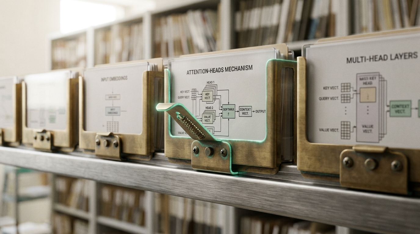
The starting observation was not made by opening the network at all. Training loss on tokens deep in a long context, as opposed to tokens near the start, showed an unusually sharp, localised improvement early in training across many models of different sizes — a pattern specific enough to demand a mechanistic explanation rather than a statistical one. The mathematical framework for transformer circuits supplied a candidate: in a two-layer attention-only model, one head’s output can feed a second head’s query or key before the second head acts, a composition the framework calls K-composition, and that composition is expressive enough to implement a concrete algorithm — find the most recent earlier occurrence of the current token, and predict whatever token followed it there ^[4].

That is a hypothesis about two specific components, and step one is to look for it. Extracting and inspecting attention patterns — the simplest activation available, already a probability distribution over positions — on synthetic sequences of repeated random tokens lets a researcher check a narrow, hand-designed signature directly: does a given head, at the current token, place its attention weight on the position that followed an earlier occurrence of that same token? Olsson and colleagues ran this check at scale, across thirty-four transformers spanning several orders of magnitude in size, and found heads carrying exactly that signature appearing at a training-time phase change that coincided with the sharp loss improvement noticed at the outset ^[5]. That coincidence in time is itself only a correlation. What made the case rather than merely suggested it was closing the loop with intervention: ablating the candidate heads — over fifty thousand individual head ablations run across the model set — substantially degraded in-context learning specifically, architectural changes that shifted when the heads could form shifted the in-context-learning improvement to match, and the mechanism generalised from tiny models to the point of varying continuously into much larger ones ^[5]. Later work sharpened the localisation further with path patching, isolating specifically the connection between a first head’s output and the second head’s key rather than the heads’ broader activity, refining “these two heads matter” into “this specific path between them carries the effect” ^[12].

Sparse decomposition adds a layer of resolution the whole-head account does not have on its own. A single attention head is a coarse unit — it can be involved in several distinct computations at once — and training dictionaries directly on attention-layer outputs rather than on individual heads found several distinguishable families of features living inside the same heads, including one cluster specifically tied to the copy-forward behaviour the induction mechanism depends on, sharpening what the ablation studies had identified only at the level of a whole component ^[10].

Assembled, the account has a name — a two-head circuit, one “previous-token” head whose job is to write the identity of the immediately preceding token somewhere a later computation can read, composing via K-composition into a second, “induction,” head whose query effectively asks what came after the thing that looked like the token before this one, and whose output copies the corresponding token forward — and it has the property that distinguishes a tested circuit from a plausible story: every link in it was checked by extraction, sharpened by decomposition, and confirmed by an intervention that would have failed to produce the predicted effect had the story been wrong. That is what “we found a circuit” is supposed to mean, and it is also, by the field’s own account, one of the few mechanisms that have been checked this thoroughly.

A second case, run to completion

The induction-head account is unusually well supported and still incomplete — a partial account of one mechanism inside models with vastly more behaviour than this one circuit. It is worth closing with a case where the same four-stage pipeline was run against a target small enough that “complete” was actually achievable, because it shows what the toolkit produces at its best rather than at its most realistic.

Nanda and colleagues trained small transformers on nothing but modular addition — predicting $(a+b) \bmod p$ for a fixed prime $p$ — a task deliberately chosen because the textbook answer to “what algorithm does this” is fixed and checkable in advance, and studied networks that grok: memorising the training set first, with poor generalisation, and only much later transitioning sharply to a solution that generalises, often long after training loss has already bottomed out ^[15]. Extraction and probing came first, applied to the network’s own weights and intermediate activations, and revealed something a probe alone could not have guessed going in: the trained embeddings organised inputs by their residue around a circle, one circle frequency per output logit, rather than in the sparse-lookup structure a memorising solution would use. Decomposing the network’s Fourier-domain activity — a spectral rather than a sparse-dictionary decomposition, but playing the same structural role of breaking a tangled representation into legible parts — showed a circuit computing sums and differences of trigonometric identities across those frequencies, an algorithm with a closed mathematical form that can be checked against the network’s actual weights term by term, not merely inferred from behaviour.

The intervention stage is where this case earns the label “run to completion” rather than merely “well supported”: because the full algorithm was known in closed form, the researchers constructed progress measures — quantities computed directly from the weights, tracking how strongly the trigonometric circuit was implemented — and showed these measures rose smoothly through the memorising phase, well before test accuracy showed any sign of the eventual jump, meaning the mechanism was demonstrably forming before its behavioural signature appeared at all ^[15]. That is a stronger claim than anything available for the induction head, and it is only available because the model organism was chosen small enough for ground truth to exist. The honest reading is not that grokking work has solved interpretability and induction heads have not; it is that model organisms buy completeness by giving up realism, and the two cases in this article sit at opposite ends of that trade on purpose.

What the toolkit does not give you

None of the above should read as a claim that this pipeline, run correctly, settles every question one might ask about a network. It settles a specific kind of question: whether a hypothesised, narrowly specified mechanism is doing the causal work its proponents say it is, on the inputs it was tested on. It says much less about whether a network has some property nobody has thought to test for, and it says close to nothing about behaviour far outside the distribution the intervention was run on — a patched activation and an ablated head test the hypothesis that was written down, not every hypothesis that could have been written down. Extraction and probing are cheap and can find structure a probe has enough capacity to invent; sparse decomposition can reconstruct an activation faithfully in a basis the network itself never uses; and even a well-designed patching experiment tests the protocol that was chosen, which is exactly why the field has moved toward reporting corruption method and metric explicitly rather than a single localisation number. None of this is a reason to distrust the toolkit — every stage exists because researchers found the failure mode of the stage before it and built a check for it — but it is a reason to read “we found the circuit for X” as a claim bounded by what was actually tested, not a general theory of what the network is doing.

Predictions, with what would falsify them

These are forecasts, separated from the sourced material above. Horizon: 12 August 2029. Assumptions: continued publication of interpretability methodology by frontier labs and academic groups, and no architectural break from the transformer that would obsolete the toolkit described here.

One. Sparse decomposition trained directly on attention-layer and cross-layer objects, rather than only on residual-stream snapshots, will become the default starting point for a new circuit-hunting project, because it hands the causal-intervention stage a shorter and more specific list of candidates than whole-head or whole-neuron ablation does. Disconfirmed if residual-stream-only dictionaries remain the field’s default reference point for new mechanism-hunting work at the horizon.

Two. Reported activation-patching results will increasingly specify corruption method and metric as mandatory reporting fields rather than incidental methodology, following directly from the demonstrated sensitivity of localisation claims to both. Disconfirmed if a majority of new patching-based circuit claims at the horizon still omit an explicit statement of corruption method.

Three. The number of small, purpose-built model organisms with a fully closed mechanistic account — closed in the sense the modular-addition case achieved — will grow steadily but remain a short list measured in dozens, not hundreds, because completeness requires a target simple enough for ground truth to exist at all, and most interesting behaviour does not live in such targets. Disconfirmed if fully closed accounts become common for behaviours in models with more than a few million parameters.

Four. Control-task-style validation — checking a diagnostic method against a case where the correct answer is already known, whether that is a probe’s selectivity or an automated circuit-finder’s ability to recover a hand-built circuit — will become a required step before a new interpretability tool’s results are taken as evidence, rather than an optional robustness check. Disconfirmed if new tool papers at the horizon continue to report results with no comparison against a known-answer baseline.

What to take away

The sequence is the method: extract activations and probe them to find out roughly where a property lives, decompose the messy result into a sparser and more specific set of candidates, intervene on those candidates to find out which of them the network’s behaviour actually depends on, then assemble whatever survives into a circuit and try to break it again a different way. Each stage exists to correct a specific weakness of the one before it — probing is cheap but can find structure the network never uses; decomposition sharpens the unit of analysis but does not certify it; intervention tests a specific hypothesis under a specific protocol, not the space of all hypotheses. The induction head shows what the pipeline produces against a real, messy, trained language model: a mechanism supported by every stage, still bounded by what was actually tested. The modular-addition case shows what it produces when the target is simple enough to check completely. Neither is the finished project of reading a model’s mind. Both are what actually running the toolkit, in order, looks like.