The Machine Before Electronics

The answer is the length of a wire

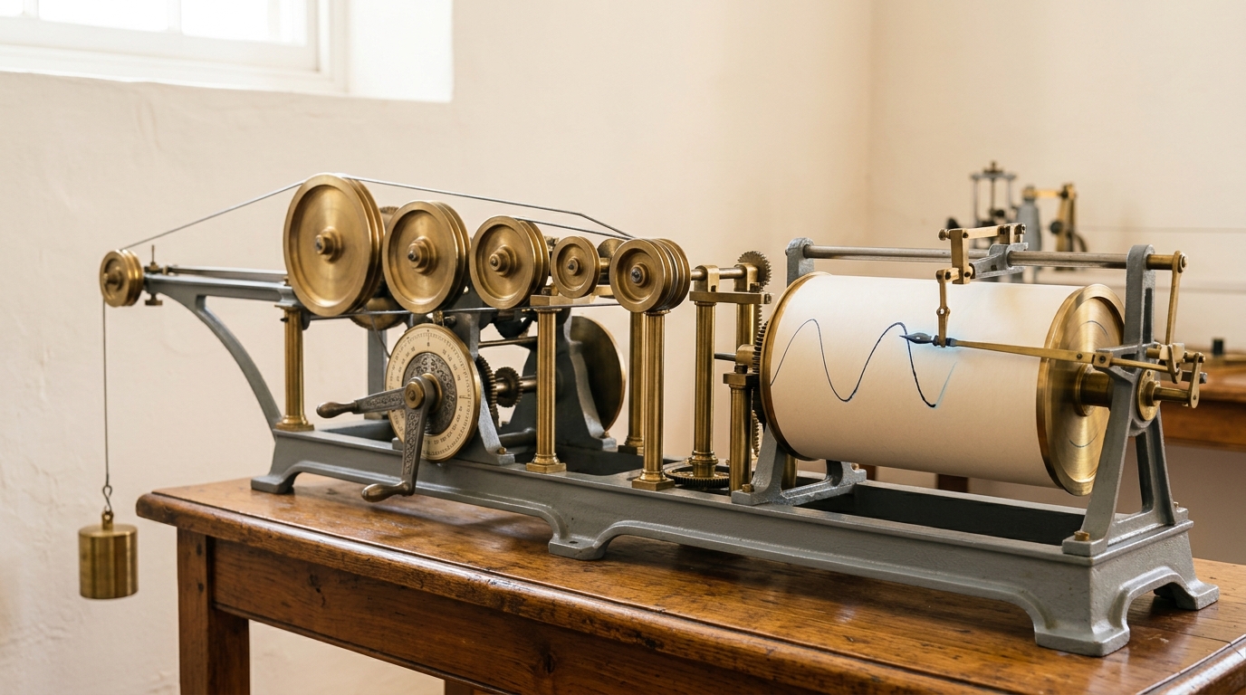
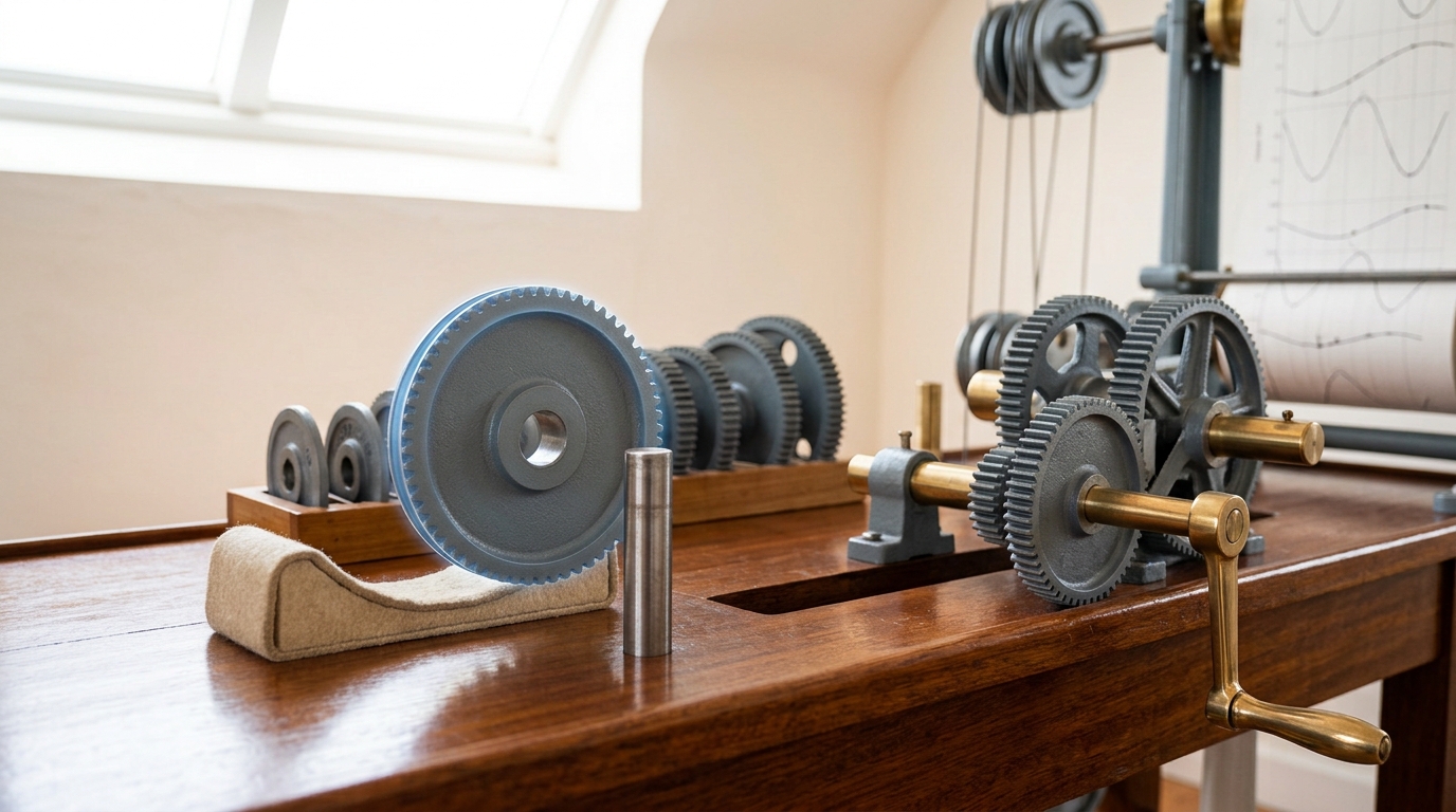
A tide-predicting machine of the kind William Thomson designed in the 1870s is a frame carrying a row of pulleys. Each pulley is mounted on an overhead crank whose throw can be set to the size of one tidal component, and the cranks are driven through gearing so that their periods stand in the ratios of the astronomical periods that raise the tides. A cord is threaded over and under the whole row and hangs from the end. When the operator turns a handle, every crank turns at its own rate, every pulley rises and falls, and the free end of the cord moves by the sum of all those motions at once ^{[3, 1]}.

Nothing in that machine performs an addition. There is no carry, no digit, no register. The addition happens because a wire threaded over a set of moving pulleys has exactly one length, and the length is the sum of the paths it is forced to take. The pen and the paper roll at the end of the frame do not compute anything either; they only record a displacement that the mechanism already holds. The National Oceanic and Atmospheric Administration’s description of its own later machines names this component plainly as the summation chain that connects the individual constituent elements and passes their total to the recording apparatus ^[2].

This is the reason mechanical and analogue computation deserves to be treated as a tradition rather than a run of picturesque failures. It is not a clumsy anticipation of the digital computer. It rests on a different answer to a prior question — what is a number, physically — and that answer supported an operational practice that produced results people navigated ships by, laid guns by, and planned invasions by. The history is more interesting if the machines are read as an alternative that lost for identifiable reasons than as an overture to something better.

Calculation is not computation

The two words are used interchangeably in ordinary speech, and the history becomes confused when they are. Calculation is the evaluation of a specified arithmetic expression: given these numbers and this operation, produce that number. Computation, in the sense that matters here, is the mechanised production of a result from inputs by a procedure, where the procedure may involve continuous quantities, integration, iteration, sorting, or search, and where arithmetic may not appear at all.

A cash register calculates. A tide predictor computes without calculating: it evaluates a function of time by physical construction rather than by executing arithmetic on symbols. A card sorter computes without calculating in a different way again, by partitioning a population of records according to a criterion. Treating all three as approximations of the same underlying activity flattens exactly the distinctions that made each of them attractive to the people who built them.

The theoretical literature keeps the distinction alive. A survey of analog models of computation opens by noting that “analog” carries two meanings at once — computing by analogy, and working on the continuum — and that models built on these premises have their own computability and complexity theory rather than being informal approximations of the discrete case ^[12]. That is a useful corrective. The question “could a differential analyser do what a Turing machine can do” is not the only question available, and for most of the period it was not the question anyone was asking.

Charles Care’s study of the field argues that historians inherited a bias here. Analog computing, he writes, emerged from an entwinement of calculation, modelling, continuity and analogy, and the modelling applications — machines built to stand in for a physical system rather than to evaluate a formula — have been systematically under-represented in the historiography relative to the calculating ones ^[9]. If that is right, the standard story is not merely incomplete; it is skewed toward the part of the tradition that most resembles what came next.

Two ways to hold a number

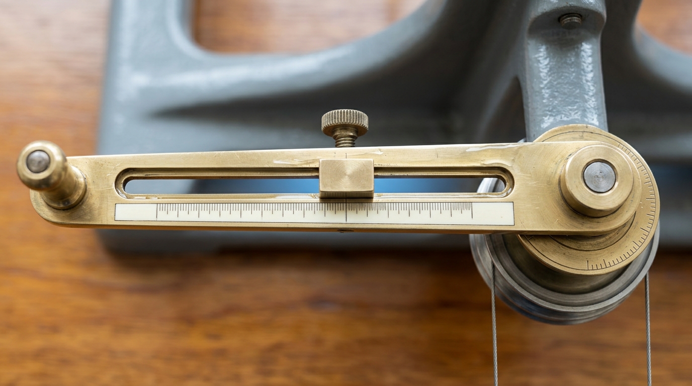
The technical distinction is about representation, and it is cleaner than the cultural one. An analogue machine represents a quantity by a physical magnitude: an angle, a displacement, a voltage, a shaft rotation, a length of wire. The representation is dense — between any two representable values there are others — and its resolution is set by the physics of the medium and the workmanship of the parts.

A digital machine represents a quantity by a configuration of discrete states: teeth on a wheel that must sit in one of ten positions, holes present or absent in a card, a relay open or closed. The representation is countable, and its resolution is set by how many states you are willing to build. Adding a digit costs another wheel or another column; adding a decimal place to a shaft angle may cost a rebuild of the whole train.

Two consequences follow, and they explain most of what happened over the following century. First, an analogue machine’s error is a property of its materials. Bearing friction, backlash, thermal expansion, cord stretch and manufacturing tolerance all enter the answer directly, and they compound along a chain of elements. There is no equivalent of rounding to a known number of places, because there are no places. Second, a digital machine can restore its own signal. A state that has drifted part-way toward its neighbour is snapped back at each stage, so error does not accumulate along the chain in the same way; the cost of that discipline is that continuous processes must first be discretised.

Neither property makes one kind of machine better in the abstract. They make each better at different jobs, which is why the two lineages ran side by side for a long time rather than one replacing the other on a schedule.

The tide predictor, worked through

Tides are the response of a rotating, irregularly shaped ocean to the gravitational forcing of the Moon and Sun. The forcing is not one periodic term but many, because the relevant astronomical cycles — lunar day, solar day, lunar month, the inclination of the orbits, the precession of the lunar nodes — beat against one another. The insight that made mechanical prediction possible was that the local water level can be written as a constant plus a sum of sinusoids whose frequencies are fixed by astronomy and whose amplitudes and phases are fixed by the harbour:

Here $\omega_n$ is a known astronomical angular frequency, while $A_n$ and $\phi_n$ are constituents determined by fitting the expression to a record of observed water levels at that specific place. The division of labour is the whole trick. The frequencies are universal and can be built into gearing once. The amplitudes and phases are local and must be adjustable.

Thomson’s machine implements exactly that division. Each of the ten shafts in the 1872 instrument carries an overhead crank with a pulley pivoted on a parallel axis that is adjustable for the range applying to that place — the amplitude $A_n$ — and each crank can be positioned and clamped to correspond to the required tidal epoch — the phase $\phi_n$. The shafts are geared so that their periods are proportional to the periods of the tidal constituents — the frequencies $\omega_n$ ^[3]. The summing cord performs the $\sum$. The pen writes $h(t)$ against a moving paper roll while a single crank drives everything at once.

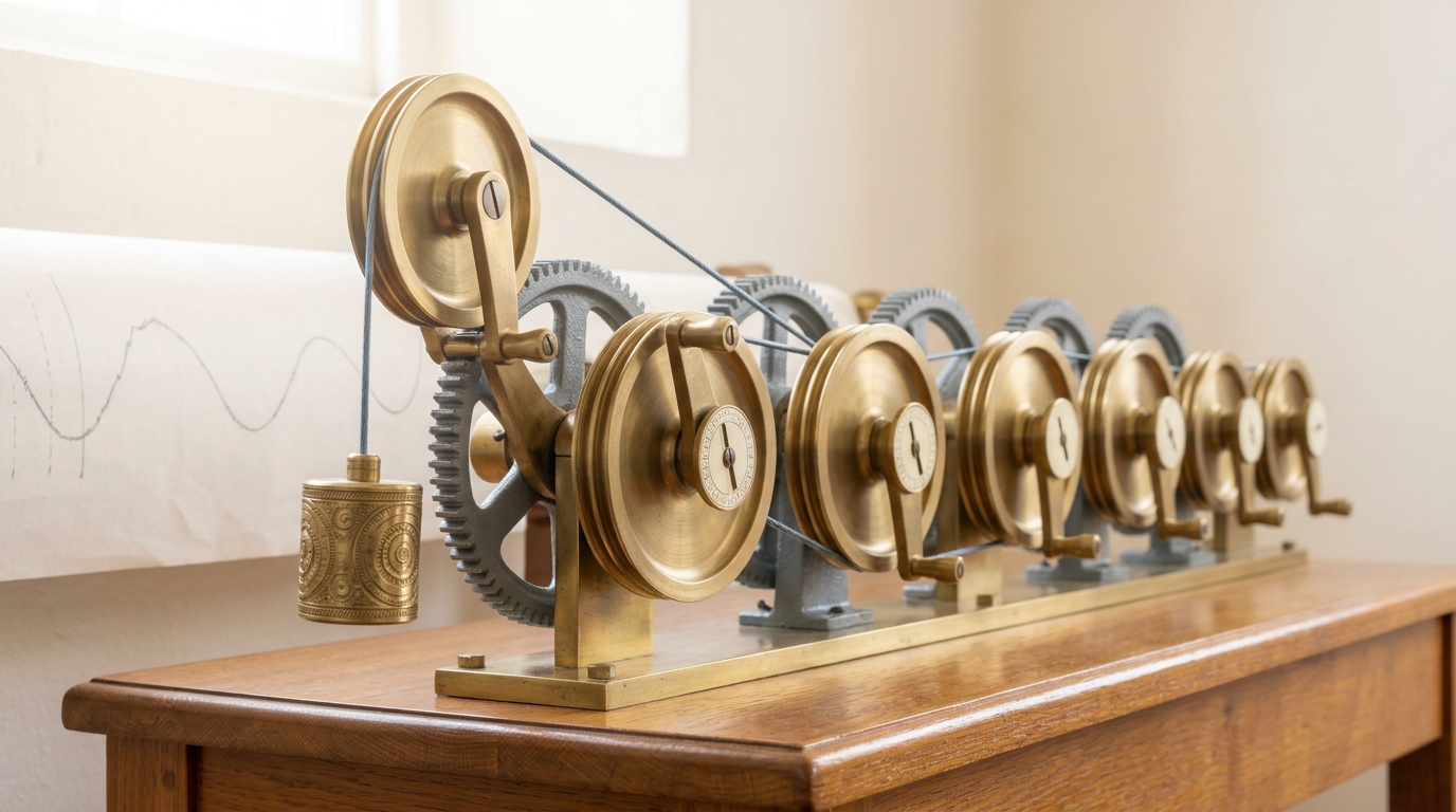
Scale followed. The first United States machine, built in 1873, provided for the summation of ten principal constituents; the Coast and Geodetic Survey’s Tide Predicting Machine No. 2, completed in 1910, was designed for thirty-seven, of which thirty-two were short-period and five long-period, and it was the first to give both the height of the tide and the times of high and low water ^[2]. Ferrel’s intermediate machine of 1874 used nineteen constituents, and Harris and Fischer’s 1910 design used thirty-seven ^[1]. More constituents meant more shafts, more gearing and more mass: the 1910 machine ran to about eleven feet long and roughly twenty-five hundred pounds ^[2].

What the machine could not do is as instructive as what it could. It could not determine the constituents; those came from harmonic analysis of observed records, a separate and laborious job. It could not predict storm surge, seiche, or any non-astronomical water level, because none of those terms exist in the model it embodies. It could not be asked a different question: a machine geared for tides computes tides. And it degraded gracefully rather than failing loudly, which is a virtue operationally and a hazard epistemically, because a slipping cord produces a plausible wrong curve rather than an obvious error.

Accurate enough to matter

The right test of an instrument is not its residual error but whether the error is small compared with the decision it informs. On that test the tide machines were decisively good enough, and the clearest demonstration is an operational one.

The Normandy landings required low water shortly after dawn so that assault engineers could clear beach obstacles before the water covered them. NOAA’s account puts the local tidal range at about twenty feet, with the water level changing roughly one foot every fifteen minutes on the flood, and notes that the predicted times differed by more than an hour across the five landing beaches spread over a hundred kilometres. A prediction error of thirty to forty-five minutes would have been enough to strand landing craft and break the reinforcement schedule. The Allies had three principal mechanical tide machines available, one in the United States and two in Britain, and the American machine — the thirty-seven-constituent instrument — had already reduced what had been about six months of hand computation to under a day ^[4].

Speed is the second half of the argument. Thomson’s 1872 machine produced a year of predictions for a port in about four hours of cranking ^{[3, 1]}. That is not a marginal improvement over hand computation; it is a change in what is worth attempting at all. Tide tables for many ports, published annually, updated as records improved, are only a routine product if the marginal cost of one more port-year is hours rather than months.

This is the pattern to keep in mind when the tradition is described as inaccurate. For a very long time these machines were not competing with an exact digital answer. They were competing with a human computer, a table of logarithms and a deadline.

Mechanical integration and the differential analyser

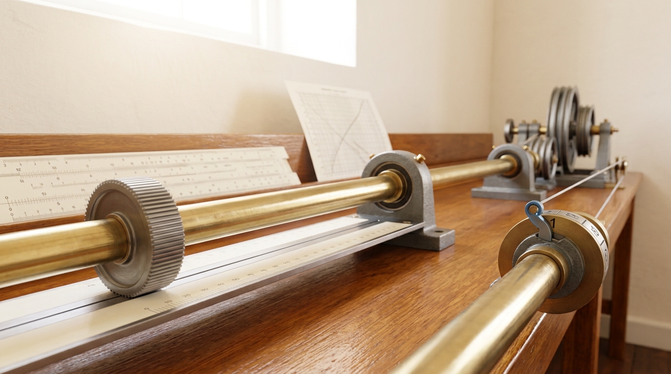
Summation is the easy operation to build. Integration is the one that opens up a whole class of problems, and the mechanism that made it practical was the wheel-and-disc integrator: a wheel riding on a rotating disc at a radius that can be varied, so that the wheel’s rotation accumulates the product of the disc’s rotation and the instantaneous radius. If the disc rotation represents the independent variable and the radial position represents the dependent one, the wheel angle represents

which is to say, the integral of $y$ with respect to $x$, produced continuously and without arithmetic.

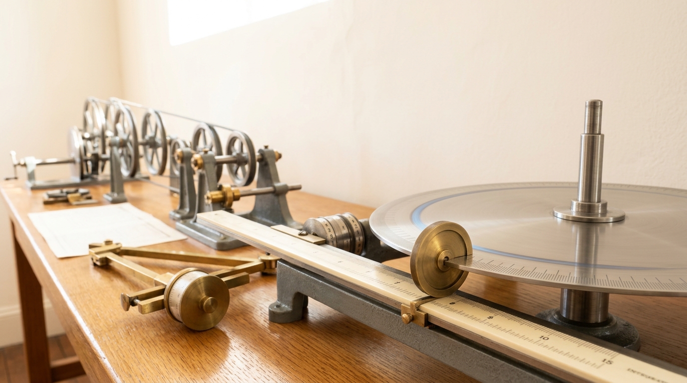
Vannevar Bush’s differential analyser, built at MIT from work begun in 1928 by his student Harold Hazen and described by Bush in 1931, put wheel-and-disc integrators at its heart and connected them through eighteen long rotating shafts driven by electric motors and a complicated array of gears. It could solve, approximately, an arbitrary sixth-order differential equation, and it was applied to problems in physics, seismology and ballistics. Copies at the Moore School and at Aberdeen Proving Ground were used specifically to compute artillery firing tables. The machine was large, needed real mechanical skill to reconfigure for each new problem, and reconfiguration was laborious ^[8].

That last clause is the seed of the whole later story, so it is worth stating precisely. Setting up a differential analyser did not mean loading a program. It meant physically re-coupling shafts so that the machine’s mechanical structure became an analogue of the equation to be solved. The machine was not instructed; it was rebuilt. The successor Rockefeller Differential Analyzer has been described as the most important computer in existence in the United States at the end of the Second World War, and it went on operating until 1954 ^[8] — a reminder that the analogue tradition was not in retreat during the years usually narrated as the birth of the digital computer.

Nomograms, slide rules and a graphical culture

Not all of this tradition was machinery. A large part of the working practice of engineering between roughly 1880 and 1970 consisted of computing by looking, and the artefacts of that practice were printed on paper.

A slide rule holds numbers as lengths along a logarithmic scale, so that sliding one scale against another adds the lengths and therefore multiplies the numbers. It is an analogue device in the strict sense: the quantity is a physical distance, and the achievable precision is set by how finely a trained eye can interpolate between engraved marks.

Nomography generalises the idea. Introduced in France by Maurice d’Ocagne in 1884, it is the study of graphical representations of functional dependencies; the resulting charts, called nomograms or alignment charts, are read by laying a straight edge across them. In the canonical three-scale form, a line joining values on two of the scales intersects the third at the answer, and the line itself is called the isopleth or index line. The scales need not be linear — they may be logarithmic, exponential, trigonometric or projected — and non-linear scales carry correspondingly varied tick density ^[7].

Two things about this deserve emphasis. First, a nomogram is a computer in the same sense a tide predictor is: the geometry of the paper embodies the relation, and the user supplies inputs and reads a magnitude. Second, its economics are extraordinary. Designing a nomogram is expensive and requires real mathematics; reproducing it costs a sheet of paper; using it requires no training beyond laying down a straight edge. Whole professions — chemical engineering, aviation, radiology, artillery — ran on chart-books that put a specialist’s derivation into a technician’s hands. The same peer-reviewed account records that this culture declined toward the end of the twentieth century as capable personal computers and handheld calculators became widespread ^[7], which is a displacement by convenience rather than by any demonstration that the charts had been wrong.

Punched cards: a separate lineage

The census tabulator belongs to a different family tree, and conflating it with calculation is one of the more persistent errors in popular accounts.

Herman Hollerith received a patent for an electromechanical tabulating machine on 8 January 1889. His system encoded records as holes punched in non-conducting cards; a hand-fed press brought wires down onto each card, and where a hole allowed a wire through into a mercury cup beneath, a circuit closed and advanced a mechanical counter or opened a bin in a sorting box ^[6]. The Franklin Institute awarded him its Elliott Cresson Medal in February 1890, following a gold medal at the 1889 Paris Exposition ^[6].

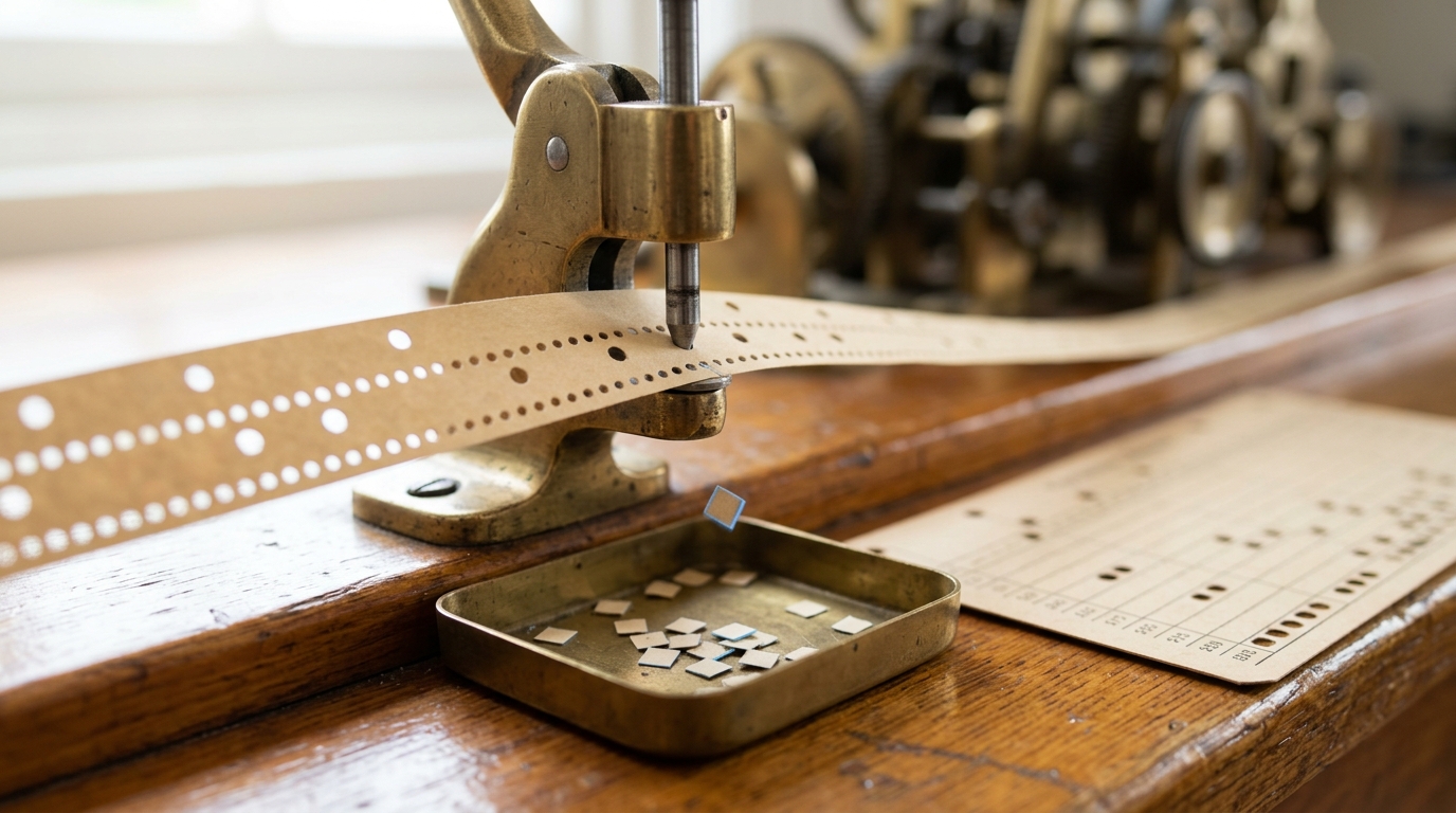
The evidence for the method was competitive rather than theoretical. In an 1888 trial on St Louis census data, two rival systems sorted the material in about forty-four and a half and fifty-five and a half hours; Hollerith’s did it in five and a half ^[5]. In service, the 1890 census completed its official population count within six months ^[6], and the Census Bureau finished publishing the 1890 results some eighteen months earlier than it had published the 1880 results, despite collecting more information ^[5]. Other national censuses adopted the system, and by 1908 it had moved into commercial and industrial work ^[6]; the Bureau went on using improved punched-card equipment into the 1950s ^[5].

Note what the machine does. It counts, sorts, and classifies. It is digital in the strict representational sense — a hole is present or absent, and there is no intermediate state — but it is not a calculator, and it is not an ancestor of the differential analyser in any useful sense. Its ancestry runs through the Jacquard loom and the filing cabinet, and its descendants are data processing, records management and the punched-card installations of mid-century business. The reason this lineage matters to the present argument is that it demonstrates that “digital” and “arithmetic” were separable from the start. The property that made cards win was not numerical precision. It was that a discrete, restorable representation can be stored, copied, mailed, re-read and re-sorted without degrading, which is a statement about media rather than about mathematics.

Where analogue stayed ahead: fire control

If the analogue tradition had simply been less accurate, it would have died quickly. It did not, and the clearest counter-example is naval gunnery, where analogue machines remained the operational standard for decades after electronic digital computers existed.

The problem is genuinely hard: a gun on a rolling ship must be aimed not at a moving target but at where that target will be after a flight time of many seconds, with corrections for own-ship motion, target course and speed, ballistic properties of the shell, wind and the Coriolis effect. The Ford Instrument Company’s Mark 1, introduced in the early 1930s, solved it as an electromechanical analogue machine. Its central element was a mechanical rate integrator — a constant-speed plate, a ball, and a second plate pressed against it — integrating time and position data in three coordinates to predict future target position. Around it sat mechanical differentials that combined inputs, synchros that carried remote data in as shaft positions, and a stable element that supplied a true horizontal reference despite the ship’s motion. The output was a continuous firing solution that removed the need to walk salvos onto the target by ranging ladders. Reliability was a design property rather than an afterthought: the machines were run without scheduled maintenance and went years without breakdown, and the Mark 1A variant of around 1935 added the dual-purpose anti-aircraft capability that carried it through the war on most United States Navy vessels ^[11].

The reasons for analogue persistence here are structural rather than sentimental. The inputs were already continuous shaft rotations and voltages, so no conversion was needed at either end. The output had to be produced continuously and in real time inside a control loop, not as a batch answer. The required accuracy was bounded by the dispersion of the gun itself, so extra decimal places bought nothing. And the machine had to survive shock, damp and salt with a crew that could not recompile anything. Mindell’s study of the interwar decades treats naval fire control alongside the Sperry Gyroscope Company, Bell Telephone Laboratories and Bush’s MIT laboratory as four distinct engineering cultures, each of which developed technologies to represent the world in a machine, and argues that the theoretical and practical foundations of control engineering and computing were laid in that period rather than emerging fully formed after 1948 ^[10].

What actually ended it

The common explanation is accuracy. That explanation is too simple, and the fire-control case is enough to refute it on its own. Two better reasons are available, and the historical actors named both.

The first is reprogrammability, and it is the decisive one. An analogue machine is a physical model of a specific problem, so changing the problem means changing the machine. On the electronic analogue computers of the 1950s and 1960s this meant patching by hand: Bernd Ulmann’s survey of the field describes programming as a complex, error-prone and time-consuming process requiring hundreds or thousands of manual connections and the careful setting of precision potentiometers, work that could take hours or days, and calls this the technology’s Achilles heel ^[13]. Set beside a stored-program machine, where changing the problem means changing a pattern of stored symbols, the comparison is not close, and it does not depend on any claim about numerical error.

The second is error accumulation. In an analogue chain, each element contributes its own imperfection to the signal, and there is no restoration step; the errors of the integrators, amplifiers, potentiometers and linkages propagate into the result and grow with the length of the computation. This is not a fixable defect of workmanship but a consequence of representing quantity by a continuous physical magnitude in an imperfect physical world. Yannis Tsividis, writing as an advocate of the technology rather than a critic, lists the properties that digital machines offered by the 1960s and 1970s — straightforward programmability, algorithmic operation, ease of storage, high precision, and the ability to handle problems of any size — and concludes that the analogue machines of the era were simply too hard to design, build, operate and maintain, being quirky instruments that needed specially trained personnel; he adds that the analogue portions of hybrid machines could not be integrated at large scale using the fabrication techniques then available ^[14].

Read together, these are arguments about the cost of change, the length of the computation and the economics of manufacture, not about whether a wheel-and-disc integrator gives the right answer. The tide machines were retired for the same kind of reason rather than for inaccuracy: NOAA’s tidal predictions moved to electronic computation in 1966, ran on mainframe hardware in the 1970s, and had migrated to personal computers by the late 1980s ^[2].

The boundary was contested at the time

It is easy to write this history as a competition between two well-defined camps. The people involved did not experience it that way, and historians of the subject disagree about how much weight the distinction should carry.

Care’s position is the strong version of the sceptical case. He argues that analog computing is best understood as a modelling technology, that analog modelling amounts to information generation rather than information processing, and that future scholarship would do better to organise itself around modelling as a category than to keep emphasising the analog-digital distinction ^[9]. Mindell’s account points in a compatible direction from a different angle: by examining four separate engineering cultures that converged only under wartime pressure, it treats “control”, “communications” and “computing” as categories that were assembled during the period rather than given in advance ^[10]. The theoretical literature keeps a third position open, in which analog models of computation are studied as legitimate models with their own results rather than as historical curiosities ^[12].

I do not think the disagreement is resolvable by choosing a winner, and characterising it is more useful. The contested question is whether “analogue versus digital” names a real technical fault line or a retrospective category that historians imposed once one side had won. The evidence pulls both ways: the representational distinction is genuine and has real engineering consequences, while the institutional and professional boundaries were blurry, hybrid machines were common and commercially serious, and practitioners moved freely between the two. A reader should be suspicious of any account — including the tidy one in the previous section of this article — that makes the outcome look inevitable from 1930.

What the tradition leaves behind

Three observations survive the period, and they are analysis rather than nostalgia.

First, representation is a design decision with costs, not a fact about nature. Choosing to hold a quantity as a displacement buys continuity, speed and zero conversion cost at the boundaries, and pays for it in drift, calibration and inflexibility. That trade has not gone away; it has moved into the analogue front ends of instruments, into sensor design and into control loops.

Second, operational adequacy is the correct standard for an instrument, and it is not the same as precision. The tide machines were used to plan an amphibious invasion at a level of error that a modern numerical model would consider crude ^[4]. They were adequate because the decision they served had a tolerance, and knowing that tolerance is the engineer’s job.

Third, the cost of changing what a machine does turned out to matter more than the quality of what it does. That is the lesson the stored-program computer taught, and it was learned against a well-functioning alternative rather than against a straw man.

There is a live claim that some of this is returning. Ulmann’s survey notes renewed interest in analogue machines as specialised co-processors as digital hardware approaches limits in energy consumption, clock frequency and integration density, and proposes automatic reconfiguration systems under digital control to remove the historical patching burden ^[13]; Tsividis argues that modern fabrication removes several of the practical obstacles that killed the earlier generation ^[14]. Those are scholarly arguments. Claims by hardware vendors that analogue silicon will displace digital accelerators for particular workloads are vendor assertions and should be held to independent reproduction before they are treated as findings; the sources cited here support only the weaker statement that serious interest has revived.

A prediction, with its conditions stated. Horizon: 2032. Assumption: that the historical diagnosis above is correct, so the binding constraint on analogue hardware is reconfiguration cost and error accumulation rather than raw accuracy. Prediction: analogue and mixed-signal computation will be adopted where the problem is fixed, the loop is tight and the precision requirement is bounded — sensing front ends, some classes of inference at the edge, specialised differential-equation solvers — and will not be adopted as a general substrate for general-purpose work. Observable indicators: whether shipped analogue accelerators are reprogrammable in software without physical re-patching, and whether independent benchmarks report end-to-end accuracy including conversion overhead rather than core efficiency alone. Disconfirmation: if a commercially deployed analogue system is independently shown to run a general, frequently changing workload at competitive end-to-end accuracy with software-only reconfiguration, the reconfiguration-cost account of why the first tradition ended is wrong, and this prediction should be discarded with it.

Until then, the honest summary is the one the machines themselves make. Turn the crank, and the wire has a length. It is a real answer, arrived at by construction rather than by arithmetic, and for the better part of a century it was the best answer anyone could get.