How We Know What Is Inside a Planet

The deepest hole is a rounding error

No one has ever sampled a planetary mantle. The deepest borehole ever drilled reached roughly twelve kilometres into a crust that is itself a thin skin on a body six thousand three hundred and seventy-one kilometres in radius. Every statement about the composition of the lower mantle, the state of the outer core, or the existence of an ocean under an ice shell is an inference, and the chain that produces it is long enough that each link deserves inspection.

That chain has a recognisable shape. A remote observable is recorded: an arrival time, a Doppler shift in a spacecraft’s radio carrier, a periodic distortion of a satellite’s shape, a magnetic field that varies at a known driving frequency. A forward model predicts what that observable would be for a given radial structure. The structure is then adjusted until prediction matches observation. What comes out is not a picture of the interior. It is the set of structures compatible with the data, filtered through whatever the forward model assumed.

This article follows that chain for real bodies, and pays particular attention to the places where it does not close cleanly.

Travel times, and the ray that never arrives

The oldest and still the strongest constraint on Earth’s interior is the time a seismic wave takes to travel from an earthquake to a station. Collect enough of those times across enough source-receiver distances and you can invert for the velocity structure that produced them, because a wave that spends part of its path in a faster material arrives sooner.

The practical form of this is a travel-time table. Kennett and Engdahl built the iasp91 tables from International Seismological Centre data recorded between 1964 and 1987, replacing the Jeffreys and Bullen tables that had been in use since 1940 ^[2]. Their contribution is instructive about what a reference model actually is. Every phase time in iasp91 derives from a single radially stratified velocity model, so the predictions are internally consistent rather than assembled phase by phase, and at teleseismic distances their P-wave times run about 0.7 seconds slower than the 1968 Herrin tables ^[2]. A shift of well under a second, across a global dataset, is the resolution at which this game is played.

The single most consequential observation in the history of the field is not an arrival but an absence. Beyond roughly 103 degrees of angular distance from an earthquake, direct P arrivals stop, and they do not resume until about 143 degrees. The gap has a simple cause: a sharp drop in compressional velocity at the core-mantle boundary bends rays strongly downward, so that a band of the surface receives no direct P energy at all. A liquid outer core explains the drop, because a liquid supports no shear and the compressional velocity falls accordingly. Inge Lehmann’s 1936 identification of weak arrivals inside that shadow, published under the title “P prime”, required a further discontinuity: a solid inner core reflecting energy back into the forbidden band.

Note the logic. The liquid outer core was not measured. It was the explanation that made a missing signal necessary rather than anomalous, and it survived because no competing structure reproduced both the shadow and the weak arrivals within it.

The whole planet ringing

Body waves are not the only seismic observable. A large earthquake sets the entire planet oscillating in discrete standing-wave modes, and those free oscillations carry information that travel times do not. A body wave samples a ray path; a normal mode samples a whole shell, weighted by its own depth sensitivity, and crucially it responds to density as well as to elastic moduli.

The modern catalogue is large. Deuss, Ritsema and van Heijst measured 196 splitting functions, 164 self-coupled and 32 cross-coupled, from 34 years of records spanning 91 major earthquakes between 1976 and 2010, including 33 modes newly sensitive to mantle compressional velocity and 10 sensitive to the inner core ^[3]. Splitting arises because a rotating, elliptical, laterally heterogeneous planet breaks the degeneracy of each mode into a multiplet, so the shape of the splitting is itself a structural measurement.

Modes and body waves do not always agree, and the disagreement is informative rather than embarrassing. Irving, Cottaar and Lekić built an outer-core model, EPOC, from normal-mode centre frequencies and found that velocity at the top of the outer core is lower than in the long-standing preliminary reference Earth model and increases more steeply with depth, while density is higher throughout ^[4]. Their model is deliberately parameterised with only three free parameters so that it is guaranteed to behave like a well-mixed homogeneous material under core conditions, and the steeper gradient removes the need for an anomalously slow layer at the top of the core that body-wave fits had appeared to require ^[4]. The reconciliation came from constraining the model class, not from adding data.

Four numbers you can get for anything

Most bodies have no seismometer and never will. For those, the inference starts from quantities obtainable by tracking alone.

Mass follows from the gravitational perturbation a body exerts on a passing or orbiting spacecraft. Radius follows from imaging, occultations or altimetry. Their combination gives mean density, which is the crudest possible interior constraint and still eliminates a great deal: a mean density near three thousand kilograms per cubic metre is incompatible with a body made mostly of iron, whatever its internal arrangement.

The fourth quantity is the one that does real work. The polar moment of inertia, normalised by mass and radius, is

and it measures how mass is distributed radially rather than how much there is. A uniform sphere has $I^{*} = 0.4$. Anything smaller means mass concentrated toward the centre; anything approaching 0.4 means a body that is close to uniform in density, which for a rocky planet means undifferentiated.

What a moment-of-inertia factor rules out is more reliable than what it establishes. It is a single number, so it cannot distinguish a small dense core under a light mantle from a larger, less dense core under a heavier one; infinitely many radial density profiles share the same $I^{*}$. But it will refuse an entire class of models outright. For Mercury, MESSENGER radio tracking combined with spin measurements gave $C/MR^{2} = 0.353 \pm 0.017$ together with a ratio of mantle-plus-crust moment to total moment of $0.452 \pm 0.035$, a combination consistent with a solid silicate outer shell over an iron-sulfide layer, a liquid iron-rich outer core and possibly a solid inner core ^[7]. Seven years later, a longer tracking arc revised the normalised polar moment to $0.333 \pm 0.005$ ^[9]. The revision is worth dwelling on: the earlier value was not wrong within its stated uncertainty, but the interior models it supported shifted materially when the uncertainty shrank by a factor of three.

Rotation is a measurement of the interior

A moment of inertia is usually not measured directly. It is recovered from how a body rotates, and rotation is sensitive to whether the interior is mechanically connected.

Mercury’s case is the cleanest. Margot and colleagues used Earth-based radar to track the planet’s rotation and found librations in longitude forced at the 88-day orbital period with an amplitude of 35.8 plus or minus 2 arcseconds ^[8]. That amplitude is roughly twice what a rigid planet would show. The interpretation is mechanical rather than statistical: if the mantle were rigidly coupled to the whole interior, the whole mass would have to be swung, and the response would be smaller. A mantle librating as though decoupled from the interior requires a liquid layer between them.

The same argument was later run on an icy moon. Thomas and colleagues measured control points across Enceladus over seven years of Cassini imaging and found a forced physical libration of 0.120 plus or minus 0.014 degrees, too large for a shell rigidly connected to the core, and large enough to require a global ocean rather than a regional polar sea ^[15].

Here the assumptions become visible. Converting a measured gravity coefficient into a moment of inertia normally proceeds through the Radau-Darwin relation, which assumes the body is in hydrostatic equilibrium. Gao and Stevenson tested that assumption against exact hydrostatic calculations and found the approximation good to better than one per cent for many plausible solid-body configurations, but also found that nonhydrostatic surface stresses of only about 0.1 bar can inflate the inferred moment of inertia by as much as ten per cent for slowly rotating bodies such as Titan, Callisto and Enceladus, while faster-rotating Ganymede requires much larger stresses to be similarly misled ^[16]. Their conclusion is not a correction to a number but a widening of the possibilities: nonhydrostatic effects could permit full differentiation of Titan and Callisto, which hydrostatic analyses had appeared to exclude ^[16].

The gravity field is a filter

A spacecraft in orbit is a gravimeter. Its along-track velocity is perturbed by mass anomalies beneath it, and Doppler tracking of the radio link records those perturbations. Expanded outside the body, the potential from a rotationally symmetric mass distribution takes the form

and the factor $(R/r)^{n}$ is the whole epistemology of gravity-based interior work. Each successive degree $n$ decays faster with altitude, so high-degree terms are measurable only from low orbit and are dominated by shallow structure. Low-degree terms reach deep but are few. A gravity field is therefore a filter that attenuates depth information in a known, unavoidable way.

For the Moon, GRAIL’s low, twin-spacecraft configuration resolved the field finely enough to recover crustal properties directly. Wieczorek and colleagues found the highland crust has a bulk density of 2,550 kilograms per cubic metre, substantially lower than had been assumed, implying an average porosity of about 12 per cent to depths of at least a few kilometres, and gave an average crustal thickness between 34 and 43 kilometres ^[10]. The porosity result matters because it decouples density from composition: rock that is lighter because it is cracked is not rock that is lighter because it is different.

For the giant planets, only low-degree harmonics are available, and the interpretation problem sharpens. Juno measured Jupiter’s even zonal harmonics $J_{2}$ through $J_{8}$ to high precision, and Wahl and colleagues found that models fit those moments best when the heavy-element core is not compact but dilute, expanded over a significant fraction of the planet’s radius, with total heavy-element content in the core region of roughly 7 to 25 Earth masses ^[17]. That range is wide for a reason the authors state plainly: the inferred structure is strongly affected by the chosen hydrogen-helium equation of state ^[17]. The gravity data are excellent; the translation into structure is only as good as the laboratory and computational physics behind it.

Saturn produced an unexpected second channel. Mankovich and Fuller showed that gravity-mode oscillations inside the planet drive waves in its own rings, so the rings act as a detector of the planet’s internal buoyancy frequency, and found the combined seismic and gravity data require a diffuse, stably stratified core-envelope transition extending to about 60 per cent of the planet’s radius and containing roughly 17 Earth masses of ice and rock ^[18]. A planet without a seismometer was made to report its own oscillations.

Tides, Love numbers and a field that should not be there

If a body is deformable, an external tidal potential distorts it, and the distortion changes its external gravity field in a way an orbiter can measure. The degree-two potential Love number $k_{2}$ quantifies that response. A rigid body has a small $k_{2}$; a body with a global liquid layer decoupling shell from interior has a large one.

Cassini flew six flybys of Titan between 2006 and 2011 with a gravity-quality radio link, and Iess and colleagues recovered $k_{2} = 0.589 \pm 0.150$, with an alternative solution of $0.637 \pm 0.224$ ^[14]. Both are far too large for a rigid ice shell over rock and are consistent with a global ocean at depth ^[14]. The measurement did not see the ocean; it measured how much the whole moon flexes each orbit, and only a decoupled shell flexes that much.

Electromagnetic induction provided the independent confirmation elsewhere. Jupiter’s tilted, rotating magnetic field sweeps past Europa at the synodic period, and a conducting shell inside the moon responds by generating an induced field opposing the change. Kivelson and colleagues used a January 2000 Galileo pass, deliberately timed so that the background jovian field orientation differed from earlier encounters, to discriminate between competing explanations, and found variations matching those predicted if a current-carrying outer shell such as a planet-scale liquid ocean lies beneath the ice ^[13]. The strength of that design is that the driving field is known, its frequency is known, and a permanent internal field cannot mimic a response that tracks the driver.

A field that is absent is also evidence

A global magnetic field of internal origin requires a convecting, electrically conducting fluid layer and a power source to keep it convecting. Its presence is therefore evidence about the thermal and compositional state of a deep layer that nothing else reaches.

Its absence is evidence too, and Mars supplies the demonstration. Mars Global Surveyor’s magnetometer, working from altitudes of 100 to 200 kilometres, found no active global dynamo but did find strong remanent magnetisation locked into the crust, with sources of multiple scales and geometries correlated with ancient highland terrain and equivalent magnetic moments reaching 1.3 times ten to the seventeenth ampere square metres ^[12]. Crucially, the largest impact basins are not magnetised, which dates the shutdown: a dynamo must have been running when the highlands cooled and must have stopped before those basins formed, placing the cessation roughly four billion years ago ^[12].

Mercury runs the argument in the other direction. A present-day field implies a liquid, convecting core now, and Genova and colleagues combined MESSENGER’s gravity and rotation solution with dynamo modelling to argue for a solid inner core with radius between 0.3 and 0.7 times that of the outer core ^[9]. This is a chain with several links: geodesy constrains bulk structure, the field constrains the fluid state, and thermal evolution modelling connects them. Each link is defensible; the composite is more uncertain than any of them alone.

Nothing inverts without a laboratory

Every inference above converts a physical observable into structure by way of a relation between pressure, temperature, composition and material properties. That relation is not derived from the planetary data. It is measured in a laboratory, at pressures reproduced by squeezing microscopic samples between diamonds and heating them with lasers, or computed from first principles and validated against those experiments.

Two results show what this input is worth. Anzellini and colleagues used fast X-ray diffraction in a laser-heated diamond anvil cell to pressures of 200 gigapascals and extrapolated the melting curve of iron to the 330 gigapascals of Earth’s inner-core boundary, obtaining 6,230 plus or minus 500 kelvin ^[5]. That single anchor point propagates outward: it sets the temperature at a known depth, which constrains the core-mantle boundary heat flux, which in turn bears on whether the base of the mantle is partially molten ^[5].

Murakami and colleagues found that magnesium silicate perovskite transforms above about 125 gigapascals and 2,500 kelvin, near 2,700 kilometres depth, into a denser phase with a stacked octahedral sheet structure, roughly 1.0 to 1.2 per cent denser than the parent, and proposed it as the origin of the D-double-prime seismic discontinuity ^[6]. Before that experiment, the discontinuity was a seismic observation without a material explanation. After it, a reflector at the base of the mantle became readable as a phase boundary whose depth depends on temperature, which turns a seismic feature into a thermometer.

The dependency runs one way and it is absolute. Without an equation of state, a measured seismic velocity is a number with no compositional meaning, and a measured mean density constrains nothing about what the material is.

Why the answer is never unique

The formal statement of the problem is old. Backus and Gilbert defined a class of observations they called gross Earth data, each of which is a single number describing the whole planet, such as its mass or the frequency of one free oscillation, and asked directly whether a finite set of such numbers determines the interior uniquely ^[1]. It does not. Their contribution was to make the failure quantitative: rather than producing one model, their method computes, for any depth, the narrowest averaging window over which the data can constrain a property, and how large the uncertainty on that average must be ^[1].

This reframes the output. An inversion does not return the density at 2,700 kilometres depth. It returns a weighted average of density over some interval around that depth, with a stated uncertainty, and the width of the interval is set by the data, not chosen by the analyst. Two structures that differ only at scales finer than that width are indistinguishable no matter how the fitting is done. Backus and Gilbert applied the machinery to exactly the case at hand: recovering a density profile from mass, moment of inertia and oscillation frequencies when the velocity profile is already known ^[1].

Three consequences follow, and they recur in every result cited in this article. Regularisation is a choice, not a neutral step; requiring a model to be smooth is an assumption about the planet that the data did not supply. Parameterisation is a prior; deciding in advance that a body has three layers rather than a continuous gradient forecloses answers before any fitting begins, which is precisely why Saturn’s diffuse core was hard to see in gravity data alone ^[18]. And a good fit is weak evidence when the model class is small, because the alternative that would have fitted better may never have been in the search space.

One station on a whole planet

The recent hard case is Mars. From 2018, InSight operated the only seismometer ever placed on another planet in working order for an extended mission, and single-station seismology is a fundamentally harder inverse problem than network seismology: with one receiver, the location and origin time of every event must be estimated jointly with the structure that the events are meant to constrain.

The published results show what one station can and cannot do. Knapmeyer-Endrun and colleagues identified at least two, possibly three, subsurface interfaces beneath the lander and reported crustal thickness of 20 plus or minus 5 kilometres if the second interface is the base of the crust, or 39 plus or minus 8 kilometres if the third is, extrapolating with gravity and topography to a global average somewhere between 24 and 72 kilometres ^[19]. Two answers, both honestly reported, with the choice between them turning on an interpretive question the data do not settle; the thicker option agrees better with surface abundances of heat-producing elements ^[19]. Khan and colleagues, using eight marsquakes with geodynamic modelling, resolved structure to 800 kilometres depth, found a low-velocity zone consistent with a thermal lithosphere much thicker than Earth’s, and predicted crustal enrichment in heat-producing elements by a factor of 13 to 20 relative to the primitive mantle ^[20].

Then the core. Stähler and colleagues detected reflections from the core-mantle boundary and, inverting them jointly with geodetic data, put the liquid core radius at 1,830 plus or minus 40 kilometres with a mean density of 5.7 to 6.3 grams per cubic centimetre, requiring a substantial complement of light elements, and concluded that Mars lacks a bridgmanite-dominated lower mantle ^[21]. They also stated the sampling limit explicitly: the seismic shadow from InSight’s position covers half the planet ^[21].

Two years later, two independent groups revised that core. Samuel and colleagues argued for an enriched molten silicate layer above the core beneath a partially molten layer, giving a smaller core of 1,650 plus or minus 20 kilometres at 6.5 grams per cubic centimetre, which requires fewer light elements and sits better with cosmochemical constraints while also explaining deep seismic phases, weak shear attenuation and the tidal response to Phobos ^[22]. Khan and colleagues, working separately, found a fully molten silicate layer 150 plus or minus 15 kilometres thick at a density of 4.05 plus or minus 0.05 grams per cubic centimetre, over a core of radius 1,675 plus or minus 30 kilometres and density 6.65 plus or minus 0.1, composed of 85 to 91 weight per cent iron-nickel with 9 to 15 weight per cent light elements including sulfur, carbon, oxygen and hydrogen ^[23].

This is the article’s central point in its clearest form. The 2021 measurement was not refuted. The reflections were real and the arrival times did not change. What changed was the model class: once a molten silicate layer was permitted in the parameterisation, the reflector that had been read as the top of the core was read instead as the top of that layer, and the core shrank by about 160 kilometres. Note also that the two 2023 groups do not fully agree with each other, differing by 25 kilometres in core radius with non-overlapping stated uncertainties, which is an honest signature of remaining systematic differences in method rather than of one group being careless.

Lunar seismology shows the same pattern on a longer timescale. Weber and colleagues applied array-processing methods to Apollo-era records decades after collection and extracted a solid inner core, a fluid outer core and a partially molten boundary layer, with roughly 60 per cent of the core liquid by volume and less than 6 weight per cent light alloying elements ^[11]. The waveforms had been on the shelf since the 1970s. The result was new because the processing was.

What would change the picture

A prediction, with its terms stated. Horizon: 2036. Assumptions: that at least one further body receives a long-lived seismometer or a dedicated tidal-gravity orbiter, and that laboratory equations of state for iron-light-element alloys and for hydrogen-helium mixtures continue to tighten at their recent rate.

Observable indicators that the prediction is tracking: published core radii for Mars converging within mutually overlapping uncertainties rather than diverging; giant-planet interior models narrowing the dilute-core mass range below its present 7-to-25 Earth-mass span as equation-of-state uncertainty falls ^[17]; and induced-field measurements at Europa yielding a joint constraint on ocean thickness and conductivity rather than the presence-or-absence result that a single flyby geometry supports ^[13].

Disconfirmation condition, stated so it can be checked: if by 2036 improved laboratory equations of state have been published and adopted while the spread across independent Mars interior models has not narrowed, then the limiting factor is not material physics but the single-station geometry itself, and the argument of this section is wrong. That would be a useful thing to learn, because it would say that no amount of laboratory work substitutes for a second receiver.

The tray is shorter than the ground

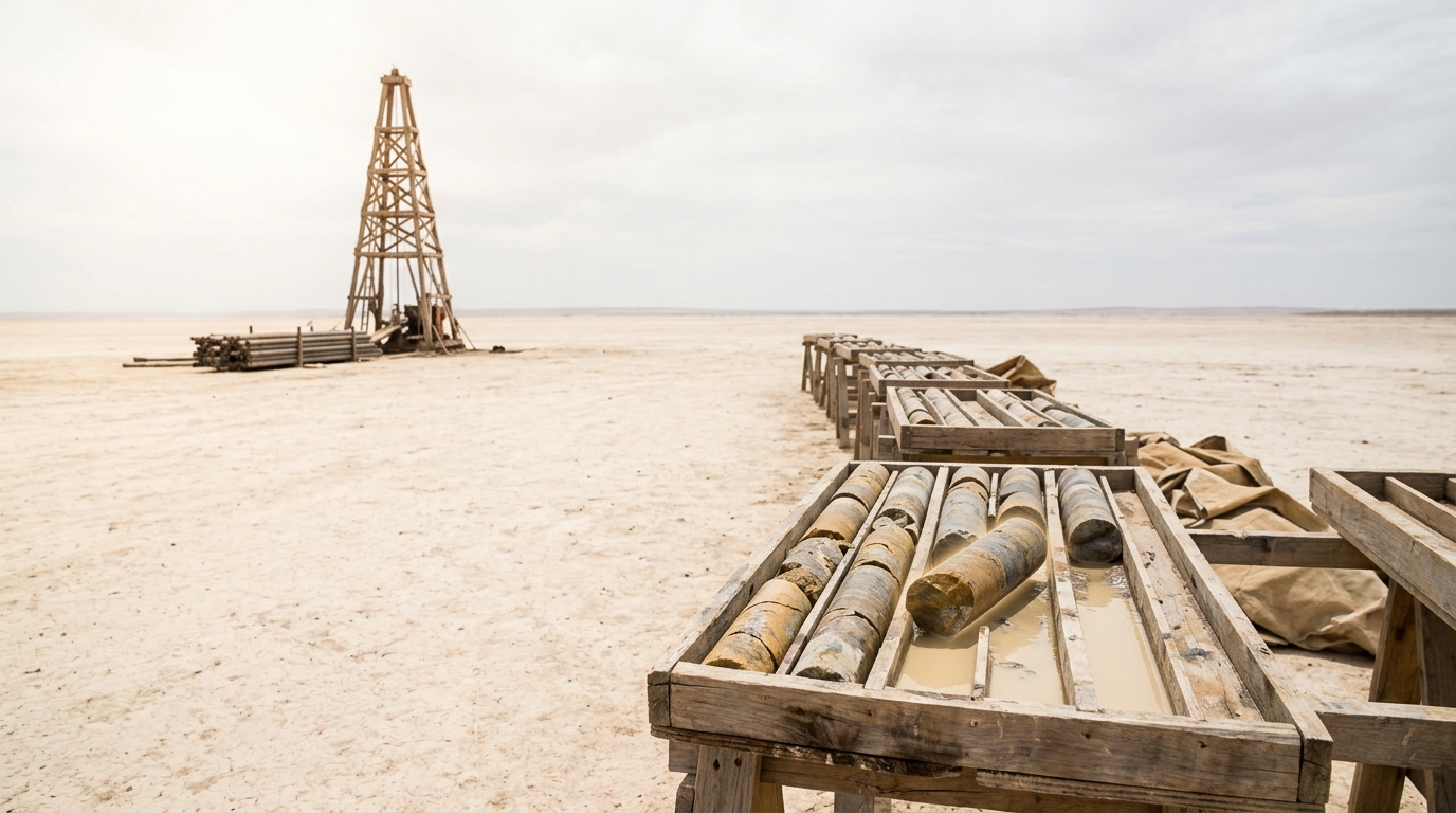
A core barrel brings up a narrow cylinder of rock, and the trays laid out beside the derrick hold a fraction of the interval drilled, with runs lost and intervals never recovered. What is written up afterwards describes a three-dimensional volume of ground. It is a real description and it is often right, but it is a reconstruction, and its reliability depends on how honestly the gaps are reported.

Planetary interiors are known the same way, on a scale where the recovered fraction is smaller still. The correct posture is neither the credulity that treats a published layer diagram as a photograph nor the scepticism that treats inference as guesswork. Between them sits the actual practice: state the observable, state the forward model, state the assumed material physics, state what the data can resolve and over what interval, and report the alternatives that fit equally well. The papers cited here mostly do this, which is why their revisions read as progress rather than as reversals.