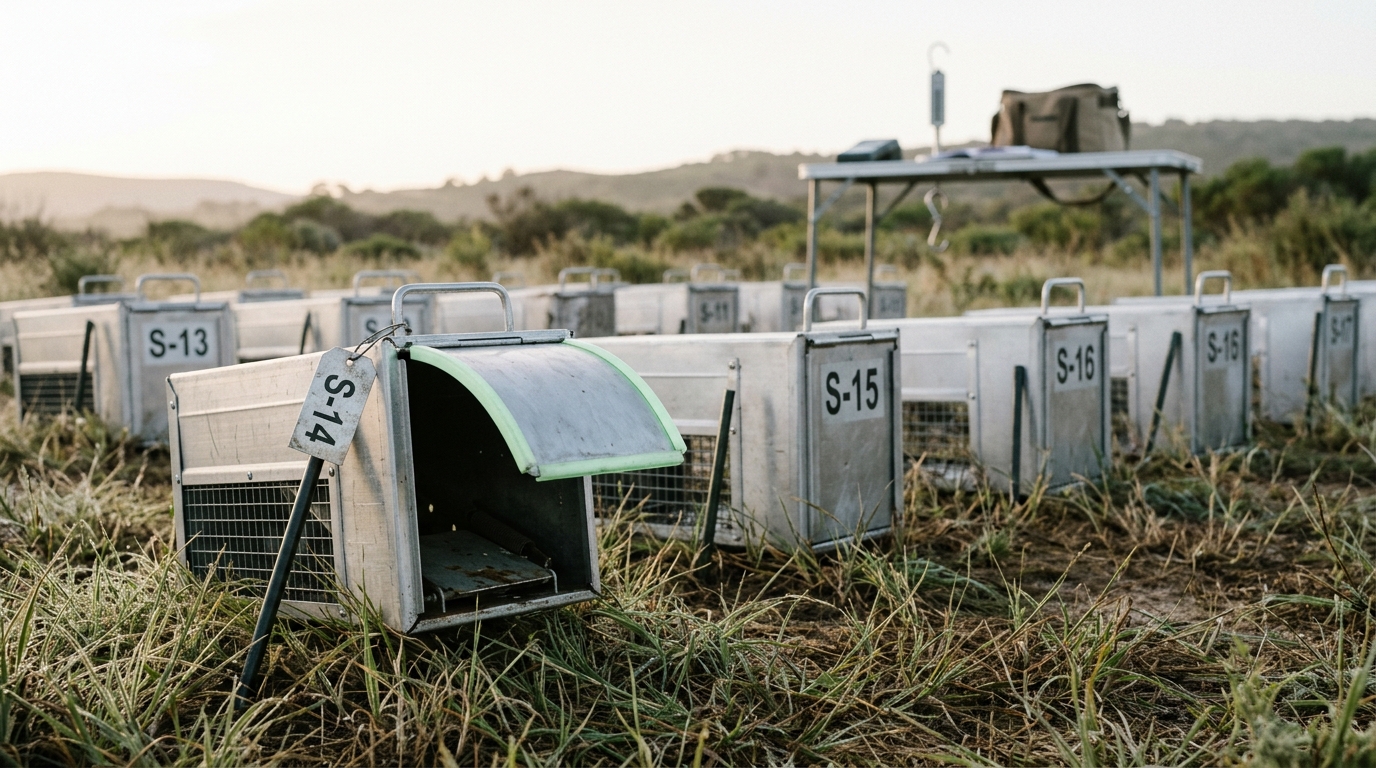
Evolutionary Biology and Ecology in Practice: An Advanced Technical Guide

Evolutionary biology and ecology are, in the field, measurement disciplines before they are theories. A claim about selection, drift, cooperation, speciation, or biodiversity loss is only as strong as the design that produced the numbers behind it, and most of the discipline’s hard-won rigor lives in three unglamorous workflows: catching and re-catching animals in a way that lets you separate “not there” from “there but missed,” extracting a population parameter from a pile of genotypes, and building a map of where a species can live that survives being checked against places it was never trained on. This guide walks through all three, using the phenomena they measure — selection, drift, adaptation, cooperation, speciation, ecosystem structure, biodiversity, and anthropogenic change — as the reason the methods exist, not as decoration around them.

Fact, convention, and inference — kept separate from the start

Before any numbers appear, a working distinction. A fact here means a specific measured value attributed to a specific study. An analytical convention is a modeling choice — an assumed mating system, a chosen kernel, a link function — that shapes the number without being itself a natural constant. A scenario is a conditional projection stated with its assumptions and an horizon. A prediction carries an explicit disconfirmation condition. Every quantitative claim below is tagged as one of these, because the discipline’s credibility problems have historically come from conflating a convention with a fact, not from the underlying biology being wrong.

Selection, drift, and the finch study that made the distinction unavoidable

The clearest field demonstration that selection and drift are both real, both measurable, and neither one predictable from the other alone comes from Peter and Rosemary Grant’s three-decade study of Geospiza finches on the Galápagos island of Daphne Major. Their 2002 synthesis in Science documented directional selection on beak morphology tracking rainfall-driven seed availability, selection reversing direction across years, hybridization altering the genetic variance selection had to act on, and population size collapsing and rebounding with drought — all in one small, closed population under continuous observation ^[1]. The paper’s own framing is instructive: evolution over that thirty-year window was not a smooth trend extrapolated from any five-year subset. A selection differential measured in one drought year predicted the following year’s mean beak depth well; it did not predict the reversal a few years later, because the direction of selection itself depended on which seed types a given rainfall pattern made available.

This matters for how the rest of this guide should be read. A single season’s mark-recapture estimate, a single population’s effective size, a single distribution model’s validation score — each is a snapshot of a system whose parameters are themselves moving. The Grant and Grant record is the fact base for treating “evolution in action” as an empirical claim rather than a metaphor: selection coefficients, generation-to-generation heritable response, and population crashes were all directly measured, not inferred from comparative anatomy after the fact.

Workflow one: designing a mark-recapture study whose numbers mean what you think they mean

The naive population estimate — mark $n_1$ animals, recapture a sample of $n_2$ later, count how many are marked, and scale up — assumes every individual in the population has the same probability of being caught in every session. That assumption is false in essentially every real population: some individuals are trap-shy, some trap-happy, capture probability drifts with weather and observer effort, and animals die or emigrate between sessions. Treating the naive ratio as ground truth silently launders all of that heterogeneity into the population estimate.

The methodological fix, formalized by Lebreton, Burnham, Clobert, and Anderson in their 1992 Ecological Monographs synthesis, is to stop estimating population size directly from raw recapture counts and instead build an explicit statistical model of the capture history — the string of detections and non-detections for each individual across sessions — with separate parameters for survival probability ($\phi$) between sessions and capture probability ($p$) within a session ^[2]. Their unified framework, built on the earlier Cormack-Jolly-Seber approach, treats $\phi$ and $p$ as estimable quantities rather than assumed constants, and — critically — provides goodness-of-fit tests to check whether the assumption that all animals of a given class share the same $\phi$ and $p$ is actually defensible for the data in hand.

Design decisions this forces on a practitioner, in the order they actually get made in the field:

1. Session spacing. Sessions must be short relative to the interval between them, so that a capture history entry can be treated as instantaneous relative to the survival process between sessions. A grid trapped for three consecutive nights each month satisfies this; a grid trapped continuously does not, because “capture” and “survival” become entangled in a single continuous process rather than separable discrete steps.

   ADVERTISEMENT

2. Trap layout and spacing relative to home range. If trap spacing is much larger than the study animal’s home range, individuals near the grid edge are captured less often not because of any biological difference but because part of their range falls outside the grid — an edge effect that inflates apparent heterogeneity in $p$ unless a buffer strip or explicitly spatial model absorbs it.

3. Marking permanence and readability. A mark that can be lost (an ear tag) or misread (a natural pattern under poor light) manufactures false non-recaptures, which the model will interpret as low survival unless mark-loss is estimated separately and subtracted out.

4. Enough recaptures to separate $\phi$ from $p$. With too few sessions, $\phi$ and $p$ are not jointly identifiable — a low apparent survival rate is statistically indistinguishable from a low capture rate. Lebreton et al.'s own case studies used designs with enough repeated sessions across enough years to break this confound; a two-session study cannot.

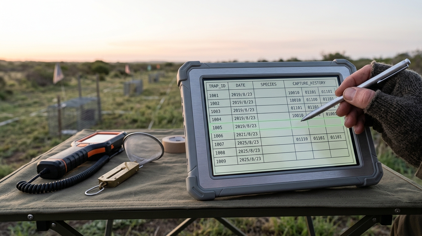
5. A goodness-of-fit test before trusting the point estimate. This is the step most often skipped under field time pressure, and it is the one the 1992 paper treats as non-optional: if the data reject the base model’s assumption of a shared $\phi$ and $p$ across individuals, the estimate from that base model is not simply “less precise,” it is potentially biased in an unknown direction, and the model needs additional structure — age classes, trap-dependence terms, or individual covariates — before its output can be reported as a population parameter at all.

The output of a well-designed mark-recapture program is not a single number; it is a survival and capture-probability estimate with a confidence interval that reflects genuine sampling uncertainty rather than an assumption stated as if it were a measurement.

Workflow two: pulling an effective population size out of allele frequencies

Effective population size, $N_e$, is not census size. It is the size of an idealized population — with random mating, no selection, non-overlapping generations, and equal sex ratio — that would show the same rate of genetic drift as the real population under study. Because $N_e$ governs how fast a population loses genetic variation and how strongly drift competes with selection, it is one of the central quantities in conservation genetics: a population with a small $N_e$ loses adaptive variation and accumulates inbreeding depression faster than its census size alone would suggest.

One of the most widely used field-deployable methods for estimating $N_e$ from a single sample of genotypes is the linkage disequilibrium (LD) method, implemented and validated by Waples and Do in their 2008 paper introducing the LDNE software ^[3]. The logic: in an infinite population at linkage equilibrium, alleles at different, unlinked loci are statistically independent — knowing an individual’s genotype at one locus tells you nothing about its genotype at another. In a finite population, genetic drift generates chance nonrandom associations between alleles at different loci purely by sampling — associations that decay each generation but are continuously regenerated by drift in a population small enough for drift to matter. The magnitude of that drift-generated linkage disequilibrium, measured across many locus pairs, is therefore a signature of $N_e$ itself, estimable from genotypes drawn in a single sampling event — no need to sample the same population twice across time, which is the main practical advantage over temporal methods.

The relationship Waples and Do build their estimator around, in the form most commonly used for the single-sample method:

where $\hat{r}^2$ is the mean squared correlation of allele frequencies across pairs of loci observed in the sample, and $S$ is the sample size, with the $1/S$ term correcting for the sampling bias that a finite number of genotyped individuals introduces into $\hat{r}^2$ even when the true population $N_e$ is large. The practical consequence practitioners have to internalize: $\hat{r}^2$ is estimated with noise from a finite sample, and that noise itself creates apparent linkage disequilibrium indistinguishable from drift-generated LD unless it is explicitly subtracted — which is exactly what the $1/S$ term does, and why the estimator is only trustworthy when the sample size and locus count used to compute it are reported alongside the point estimate, not just the final $\hat{N}_e$.

What this means for study design, working backward from the estimator:

• More independent loci reduce variance in $\hat{r}^2$ directly, because the estimator averages the pairwise correlation across many locus pairs; a handful of markers gives an estimate too noisy to distinguish a genuinely small population from sampling artifact.
• Physically linked loci must be excluded or flagged, because the method’s entire logic depends on treating background disequilibrium as drift-generated between unlinked loci; loci close together on the same chromosome carry disequilibrium from physical linkage that has nothing to do with $N_e$ and will bias the estimate upward in apparent LD, downward in inferred $N_e$.
• A single-sample estimate reflects the harmonic mean $N_e$ over roughly the last few generations, not a current instantaneous count — a fact that matters directly for interpreting a low estimate as “this population is currently small” versus “this population went through a bottleneck a few generations back and has since rebounded,” which the LD estimate alone cannot distinguish without additional temporal sampling.

The genetic estimate and the demographic estimate from workflow one are not redundant. A mark-recapture study can show a stable or growing census count while an LD-based $N_e$ estimate reveals a much smaller effective size — a mismatch that is itself diagnostic, typically pointing to high variance in reproductive success (a few individuals contributing disproportionately to the next generation) or a historical bottleneck whose genetic signature outlasts the demographic recovery.

Adaptation, cooperation, and speciation as things these tools actually measure

The same mark-recapture and genetic-sampling infrastructure that estimates $N_e$ is what field studies of adaptation and cooperation are built on. Heritable variation in a trait under selection — the beak-depth story above — requires knowing which individuals are related to which, which in turn requires either pedigree reconstruction from genetic markers or long-term individual-based mark-recapture records linking parents to offspring across seasons. Studies of cooperative behavior (helpers at the nest, alarm calling, reciprocal grooming) that invoke kin selection as an explanation are only as strong as the relatedness estimates behind them, and those relatedness estimates come from the same genotyping pipeline described in workflow two, just applied pairwise between individuals rather than population-wide.

Speciation research sits at the intersection of both workflows: incipient reproductive isolation between diverging populations is detected as elevated genetic differentiation at some loci relative to the rest of the genome — a signature that requires enough independent markers, and a clean enough separation of drift from selection, to distinguish “these two population samples happen to differ by chance” from “selection or reduced gene flow is actively maintaining a genetic barrier between them.” None of this is available without the sampling design discipline from workflow one and the estimator discipline from workflow two applied jointly and carefully.

Workflow three: building a species distribution model that means something

A species distribution model (SDM) relates a set of known occurrence locations for a species to environmental predictor layers — temperature, precipitation, elevation, land cover — to produce a predicted probability, or relative suitability, of occurrence across a landscape, including places never surveyed. Elith and Leathwick’s 2009 review in the Annual Review of Ecology, Evolution, and Systematics frames the entire enterprise around a specific danger: an SDM fit to occurrence data will always produce a plausible-looking map, whether or not the underlying data and model choices support the inference being drawn from it ^[4]. The review’s central methodological point is that “explanation” and “prediction” are different goals requiring different validation, and a model tuned for one can silently fail at the other.

One of the most widely adopted algorithms in this space is maximum entropy modeling, introduced for species distributions by Phillips, Anderson, and Schapire in 2006 ^[5]. Given presence-only data (no confirmed absences, which is the typical field situation — a species not detected at a site might simply have been missed), MaxEnt estimates the probability distribution over the landscape that has maximum entropy — is as uninformative as possible — subject to the constraint that the expected value of each environmental predictor under the fitted distribution matches its empirical average at the known presence points. This is a specific, checkable modeling assumption, not an arbitrary black box: the fitted surface is the least additional structure consistent with the presence data and the chosen predictors, which is a principled way to avoid overfitting to noise in presence-only records, but it also means the result depends entirely on which predictors were offered to the model and how well the presence points sample the environmental space the species actually occupies.

Building and validating an SDM, as it is actually done in a field-to-desk workflow:

1. Occurrence data cleaning first. Naimi et al.'s 2014 study in Ecography quantified something practitioners had long suspected: positional uncertainty in occurrence records — GPS error, coarse-resolution museum localities, digitized-from-map coordinates — measurably degrades SDM performance, with the size of the effect depending on how that spatial error interacts with the resolution of the environmental layers used ^[6]. A model built on occurrence points with unexamined coordinate precision is validated against noise it never accounts for.

2. Predictor selection with an eye to collinearity and biological relevance, not simply “add every layer available.” Elith and Leathwick’s review stresses that predictor choice should follow from a hypothesis about the mechanism limiting the species’ range — physiological tolerance, resource availability, biotic interaction — because a model built purely on statistical fit to whatever layers happen to be downloadable risks fitting incidental correlations that will not transfer to new places or times ^[4].

3. Spatially or temporally independent validation, not random cross-validation on the same occurrence set. Because nearby occurrence points tend to be environmentally similar to each other by virtue of geographic proximity, a random train/test split can appear to validate well while badly overestimating the model’s ability to predict in genuinely new locations. The stronger test — the one this article’s angle turns on — is checking predictions against occurrence records from a spatial block, time period, or survey effort the model never saw during fitting, which is precisely the discipline Elith and Leathwick’s review holds up as the difference between a model that merely fits and one that actually explains or predicts.

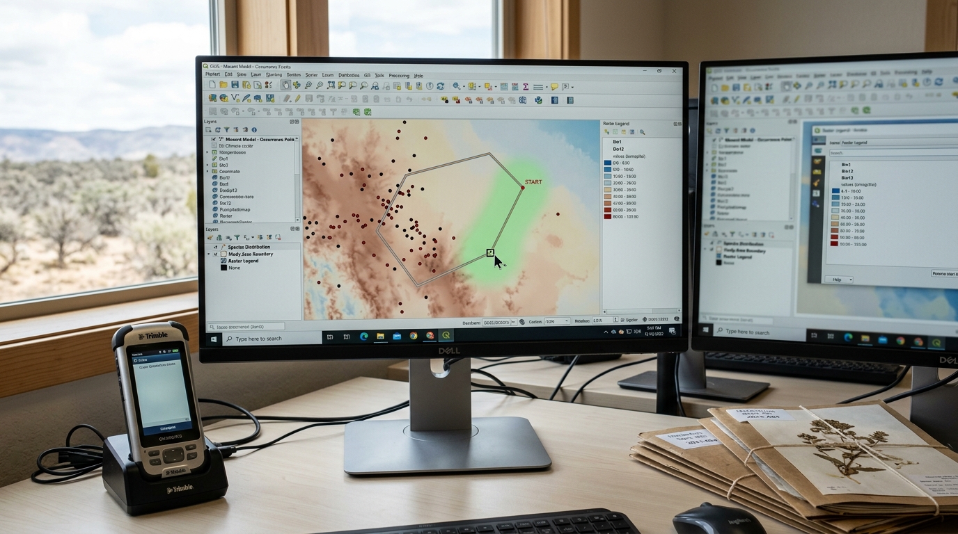
4. Reporting validation metrics against a stated purpose. A model built to predict where a species could establish under future conditions needs different validation than one built to explain which environmental variables currently limit its range; conflating the two, the review warns, is one of the most common ways an SDM’s stated confidence outruns what its validation actually supports.

Biodiversity loss and extinction: what the field record actually shows

The same population-level tools — mark-recapture-based abundance and survival estimates, genetic estimates of $N_e$ and diversity, and distribution models tracking range contraction — are the instruments behind the field’s most consequential empirical claims about anthropogenic biodiversity change. Dirzo and colleagues’ 2014 synthesis in Science compiled vertebrate, invertebrate, and plant population trend data across terrestrial ecosystems and documented widespread declines in abundance and range even among species not yet classified as globally threatened with extinction — a phenomenon the authors term “defaunation,” distinct from outright extinction because it captures functional loss (reduced pollination, seed dispersal, predation pressure) that occurs well before a species formally disappears ^[7]. Ceballos, Ehrlich, and Dirzo’s 2017 follow-up in the Proceedings of the National Academy of Sciences quantified this at larger scale, analyzing range contraction and population loss across thousands of vertebrate species and concluding that population-level declines are far more widespread than species-level extinctions alone would indicate — describing the pattern as a “biological annihilation” already underway rather than a future risk ^[8].

These are facts about measured trends, attributed to the specific datasets and time windows the two papers analyzed; they are not, by themselves, a prediction about any specific ecosystem’s future trajectory. Where this article ventures a forward-looking statement, it is marked as such: scenario — if current land-use conversion and hunting/harvest pressure documented in these two studies continue at approximately their 2010s rates, the functional declines Dirzo et al. describe as already underway would be expected to continue accumulating over the next few decades, particularly among larger-bodied vertebrates whose population growth rates are slowest to recover. This scenario’s assumptions are: continuation of currently documented land-use and harvest trends, no major new conservation intervention at the scale needed to reverse them, and no large climatic disruption reordering which species are most affected. Its disconfirmation condition is explicit: a sustained reversal in the specific population-trend indices used by either paper’s underlying datasets (such as the Living Planet Index-style trend series Ceballos et al. draw on) over a comparable multi-decade window would falsify the scenario as stated.

Where practitioner judgment cannot be automated away

Across all three workflows, the recurring lesson is the same: the statistical machinery — capture-history models, LD-based $N_e$ estimators, maximum-entropy distribution surfaces — is only as trustworthy as the design decisions made before any data are collected and the validation decisions made after a model is fit. A goodness-of-fit test that is skipped, a linked-locus pair left in an $N_e$ calculation, or a distribution model validated against its own training region rather than an independent one will each produce a number that looks exactly like a real estimate and is not one. None of the peer-reviewed methods surveyed here promise to remove that judgment; each one exists specifically to make the judgment checkable, by supplying a diagnostic — a goodness-of-fit statistic, a sample-size correction term, a spatially independent validation score — that turns “trust the estimate” into “here is the test the estimate had to pass.”