Einstein's Random Walk and the Mathematics of Genetic Drift

A Fluctuation Becomes a Measurement

On 11 May 1905 Albert Einstein submitted a paper to Annalen der Physik that had nothing to do with relativity or light quanta, the two ideas that would make that year famous. It opened instead with a claim about pollen grains: “bodies of a microscopically visible size suspended in liquids must, as a result of thermal molecular motions, perform motions of such magnitude that they can be easily observed with a microscope” ^[1]. Einstein added, tellingly, that he was not sure this was the already-known phenomenon called Brownian motion — “the data available to me on the latter are so imprecise that I could not form a judgment on the question” ^[1]. He had derived the effect from theory alone, from nothing more than the assumption that heat is molecules in motion, without first checking what the microscopists had already reported.

Working through the statistical mechanics of a wall permeable to solvent but not to suspended particles, Einstein arrived at a differential equation for how the concentration $f(x,t)$ of particles along one axis changes over time:

the diffusion equation, in a form still written the same way today ^[1]. Solving it for particles released from a point gives a spreading distribution whose variance grows linearly, not with the square root of time as a naive guess might suggest but as

with the diffusion constant $D$ fixed by measurable quantities. Einstein derived it explicitly, from the balance between the drag on a sphere of radius $P$ in a fluid of viscosity $k$ and the osmotic pressure driving diffusion, as

where $R$ is the gas constant, $T$ the absolute temperature, and $N$ Avogadro’s number ^[1]. That last dependency was the trap door: if $D$ could be read off a microscope by timing how far a particle wandered, and every other term in the equation was already known independently, then watching one particle jiggle became a way to count atoms.

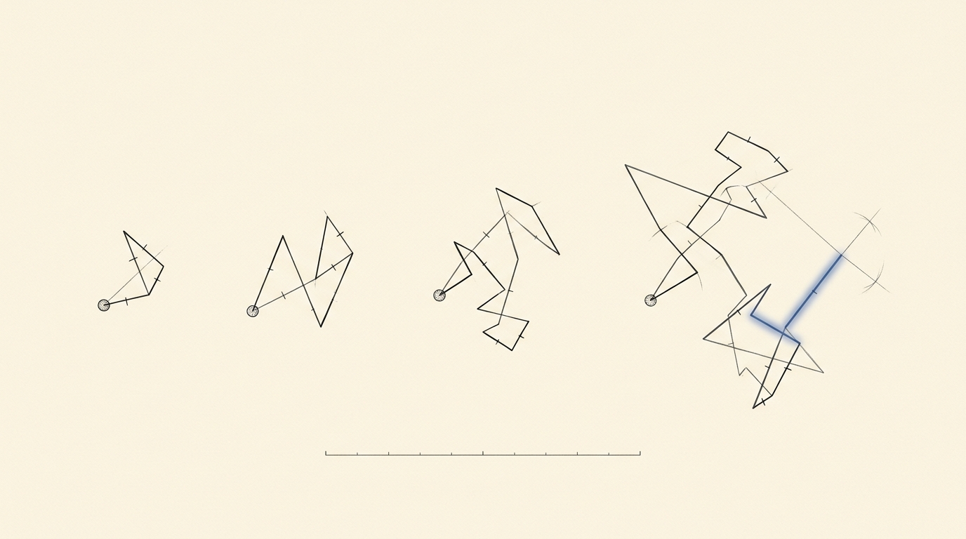
Jean Perrin spent 1908 to 1913 doing exactly that, working with Joseph Ulysses Chaudesaigues to track suspended particles under a microscope, marking each one’s position at fixed intervals and turning the resulting zig-zag tracks into statistics of displacement ^[2]. The values of Avogadro’s number he recovered agreed with figures from entirely unrelated methods in the kinetic theory of gases and radioactive decay, a convergence that settled a decades-old dispute over whether atoms were real objects or a convenient bookkeeping fiction ^[2]. The 1926 Nobel Prize in Physics went to Perrin for work its citation credits with putting “a definite end to the long struggle regarding the question of the physical reality of molecules” ^[2].

The Random Walk Gets a General Law

Einstein’s equation described one physical system: particles buffeted by a fluid held at a fixed temperature, governed by a single constant $D$. Within a decade, physicists working on an unrelated problem — how the energy of a rotating electric dipole settles under both random radiative kicks and a systematic damping force in a radiation field — found they needed the same mathematical object with one addition: a drift term standing alongside the diffusion term. Adriaan Fokker wrote down that generalization in 1914, and Max Planck rederived and extended it in 1917; the combined equation has carried both names since ^[3]. In one dimension it reads

where the first right-hand term carries the probability density along a deterministic drift $\mu(x,t)$ and the second spreads it by diffusion at rate $D(x,t)$ ^[3]. Andrei Kolmogorov arrived at the identical equation independently in 1931, from pure probability theory, as the forward equation governing how the probability distribution of any continuous-time Markov process evolves ^[3]. Kolmogorov’s work also produced a companion equation, run backward in time from a fixed outcome rather than forward from a fixed start, that turns out to be the more convenient tool for asking what a process is heading toward rather than where it began — a distinction that mattered when the same mathematics was pointed at a population instead of a particle. That third, unrelated derivation is what turned Einstein’s equation from a fact about pollen grains into a piece of mathematics indifferent to what its variable represents — a state of affairs population genetics was about to test.

The Same Equation Learns to Count Genes

Indifference to subject matter is a strong claim, and Ronald Fisher made the first attempt to cash it out for biology. His 1922 paper “On the Dominance Ratio” treated the frequency of a gene in a finite population as a continuously distributed random variable obeying a differential equation of exactly this drift-and-diffusion form — a genuine, if flawed, first pass at what a physicist would already have recognized ^[4]. The flaw was real: Fisher assumed the mean change in his transformed frequency variable was zero across generations, which produced a rate of loss of genetic variability of 1 in 4N per generation rather than the correct 1 in 2N ^[4]. Sewall Wright found the error around 1925 and, in his own 1931 paper “Evolution in Mendelian Populations,” worked out the joint stationary distribution of gene frequencies under mutation, migration, selection, and drift acting together, in essentially the form still used today ^[5]. Wright’s paper is also where the diffusion picture picked up the parameter that lets it apply to a real, structured population rather than an idealized one: effective population size, a count of breeding individuals corrected for unequal sex ratios, variable family size, and population subdivision, substituted for $N$ wherever the equations call for the census size ^[5]. Fisher corrected his own treatment in 1930, this time building explicitly on the Fokker-Planck equation borrowed from physics ^[4].

Motoo Kimura, at Japan’s National Institute of Genetics, made the borrowing exact rather than approximate. His 1955 paper in the Proceedings of the National Academy of Sciences solved the full time-dependent diffusion equation derived from the Wright-Fisher model, recovering not just the eventual resting distribution of an allele’s frequency but its whole transient shape as it evolves generation by generation ^[6]. His 1962 paper in Genetics then posed the general fixation problem as a diffusion boundary-value equation and named the lineage precisely: the question of a mutant gene’s ultimate fate was “first treated quantitatively by Fisher (1922),” with “equivalent results” reached independently by Haldane in 1927 and Wright in 1931 ^[7]. Kimura wrote the fixation probability $u(p,t)$ as the solution of what he explicitly called the Kolmogorov backward equation, subject to the boundary conditions $u(0,t)=0$ and $u(1,t)=1$ — an allele already lost stays lost, one already fixed stays fixed ^[7]. That boundary structure is doing real work: it is the diffusion equation’s way of encoding that zero and one are absorbing states of a finite population, not just convenient endpoints on a graph. Set the two founding equations beside each other and the claim of one shared mathematics stops being a figure of speech:

The same second-derivative operator acts on a diffusion term in both; only the variable and the coefficient it multiplies have changed. One honest difference is worth stating rather than smoothing over: Einstein’s $D$ is a constant, fixed once by temperature and viscosity, while Kimura’s $V(p)$ depends on the frequency itself, so the spread is fastest near $p=0.5$ and vanishes at the boundaries — an allele already fixed or already lost has nothing left to drift into ^[7]. The operator is identical; the coefficient it acts on has learned something about the biology.

That machinery pays off in the cleanest result in the theory of drift. Kimura’s 1962 formula for the probability that a gene with selective advantage $s$ eventually fixes, starting from frequency $p$ in a population of effective size $N$, is

as verified directly from his derivation ^[7]. Let the selective advantage vanish — the allele is neutral, indistinguishable from its alternatives in its effect on survival or reproduction — and the exponentials cancel term by term, leaving

The probability that a neutral allele eventually takes over the population is exactly its own starting frequency, nothing more. No fitness calculation, no bookkeeping of selection coefficients, is needed to answer the single most consequential question about a new mutation’s fate; the diffusion equation alone answers it.

A Second Fluctuation Confirms a Second Theory

Perrin’s microscope gave Einstein’s equation the ending every prediction wants: a measurement nobody could argue with. Genetic drift in a wild population has no equivalent camera — nobody photographed an allele’s frequency wandering through the Pleistocene. But the mathematics still made a testable prediction, and a different fluctuation supplied evidence for it. Comparing hemoglobin and other protein sequences across mammals in the early 1960s, Emile Zuckerkandl and Linus Pauling found that the number of amino-acid differences between two species’ proteins grows roughly in step with the time since those species last shared a common ancestor, and by 1965 had generalized the finding into a molecular evolutionary clock ticking at a roughly constant rate ^[11]. Kimura treated that near-constancy as load-bearing evidence rather than a curiosity: an evolutionary rate driven mainly by selection should track how strongly each protein’s function matters and should vary sharply between genes and lineages under different selective pressures, while a rate driven mainly by neutral drift is set by the mutation rate alone and is expected, to first approximation, not to depend on population size at all — closer to the near-uniform ticking the protein data actually showed ^[9]. Kimura restated this evidentiary case in his own later survey of the field, opening it by contrasting the neutral theory directly against “the Darwinian theory of evolution by natural selection” on exactly this point of what fixes most molecular variants ^[8].

Where Perrin’s numbers matched three independent physical methods to a stated precision, the clock’s confirmation of drift was always a looser, statistical regularity — and later work has made that looseness explicit rather than resolving it away. A 2014 review of molecular-clock methods states plainly that “lineage effects cause most genetic data to exhibit significant departures from the strict” clock, driven by differences in generation time, metabolic rate, and DNA-repair efficiency between lineages, compounded further by gene-by-lineage interactions that vary the pattern again from one gene to the next ^[10]. Modern phylogenetics answers this overdispersion with relaxed-clock models — some letting a lineage’s rate correlate with its parent’s, others treating each branch’s rate as an independent draw — that let the substitution rate wander around its neutral expectation rather than assuming Kimura’s original near-constancy outright ^[10]. The clock confirmed the theory it was built to test, but never as cleanly as a microscope confirms a diffusion constant: Perrin was checking a single fixed number against theory, while the clock’s defenders were, and still are, checking a statistical average against a mathematical idealization that no single lineage obeys exactly.

One Mathematics, Two Sciences

One differential operator organizes both a jiggling grain of resin and a gene pool’s allele frequency, and not by resemblance chosen for a reader’s benefit — the two systems are not “like” each other the way a genome is loosely “like” a computer program, an analogy picked for intuition rather than mechanism. Both are literal instances of the same limiting mathematical object: a quantity that changes, collision by collision or generation by generation, by the sum of a very large number of small, independent, additive perturbations — water molecules striking a particle from random directions in one case, the binomial lottery of which gametes happen to be sampled into the next generation’s finite pool in the other. Whenever that condition holds, the continuous-time limit of the process is forced into drift-diffusion form regardless of what is doing the perturbing, for the same structural reason a sum of many independent small errors is forced toward a bell curve regardless of what is generating the errors: this is the same limiting mechanism, at bottom, that the central limit theorem describes for a single sum, generalized from one final total to the whole evolving path of running totals. Physics and genetics did not converge because someone noticed a clever metaphor between particles and populations; they converged because the underlying mathematics, being a statement about accumulation under independence rather than about pollen or genes specifically, was never in a position to notice which one it was describing.

A loose analogy would have stopped at the word “random”: both processes involve chance, so both get called a random walk, and the resemblance ends where the metaphor stops being convenient. A formal analogy goes further and insists on the correspondence term by term — a state variable, a drift coefficient, a diffusion coefficient, a pair of boundary conditions — and demands that solving one equation solve both problems at once, which is exactly what happened when Kimura’s boundary conditions turned out to be Einstein’s diffusion equation with absorbing walls added. That is what a formal analogy done right looks like, and it is the reason a page of Kimura’s diffusion equation and a page of Einstein’s, with the axis labels covered, are the same page with $x$ renamed $p$.