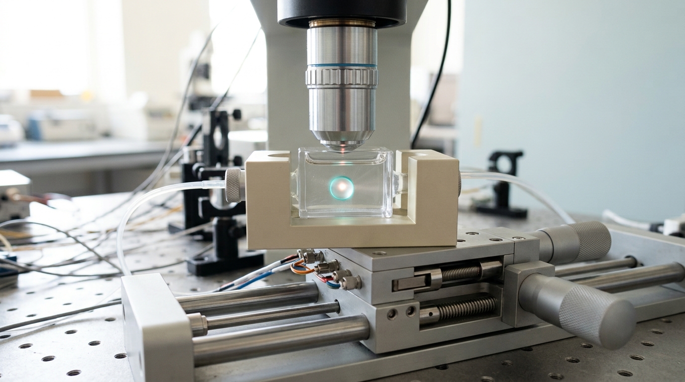
A single strand of RNA held between two optical tweezers, a swarm of self-propelled colloidal particles crowding a microscope slide, and a molecular motor stepping along a filament are three completely different physical systems that nonequilibrium statistical physics claims to describe with a shared vocabulary — work, heat, entropy production, dissipation. That vocabulary comes from at least three distinct theoretical frameworks, developed on different timelines by different communities, and the frameworks answer different questions. Conflating them is the most common mistake in secondary treatments of this field, and it happens because all three frameworks quantify “how far from equilibrium” a process runs, using overlapping notation, on the same class of systems.
This article separates the three main approaches on comparable terms: fluctuation-theorem methods built around the Jarzynski equality and the Crooks relation [1] [2]; the broader entropy-production accounting of stochastic thermodynamics [3]; and large-deviation theory, which quantifies the probability of rare fluctuations directly [4]. None of the three is a general replacement for the others. Each was built to answer a specific question, each has a specific data appetite, and each has been tested against a specific class of experiments. Treating any one as a universal nonequilibrium toolkit — a habit visible in some popular-science coverage and in overreaching grant language — overstates what a single result actually licenses.
What “nonequilibrium” is being measured, concretely
Before comparing frameworks it helps to fix the object all three are trying to describe: a small system — a stretched biomolecule, a driven colloidal particle, a molecular motor, a network of coupled chemical reactions — coupled to a heat bath and pushed away from thermal equilibrium by an external protocol or a continuous energy source. Because the system is small, thermal fluctuations are not negligible background noise; they are comparable in size to the quantities of interest. Work, heat, and entropy production become random variables with their own probability distributions, not single numbers. That is the shared starting point. What differs is what each framework does with those distributions.
Fluctuation theorems: equilibrium information from nonequilibrium driving
The Jarzynski equality states that averaging the exponential of negative work over an ensemble of nonequilibrium trajectories — trajectories driven arbitrarily fast and far from equilibrium — yields exactly the equilibrium free-energy difference between the start and end states [1]. The Crooks fluctuation theorem sharpens this into a relation between the full forward and reverse work distributions, showing they cross at the point where work equals the free-energy difference [2]. Both results are exact identities for systems obeying microscopically reversible dynamics; they carry no small-perturbation assumption, which is what makes them useful for processes driven far too fast for linear-response theory to apply.
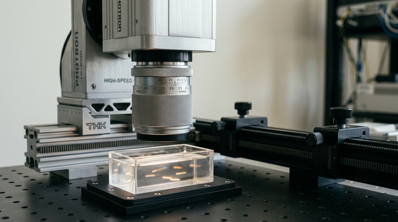
Their scope of applicability is narrow but well defined: single-molecule pulling and unfolding experiments, where a molecule is repeatedly driven between two configurations under controlled protocols and its work can be measured on each repetition. The equality was verified directly by mechanically stretching single RNA hairpins reversibly and irreversibly and recovering the known folding free energy from the nonequilibrium work distribution [5]; the Crooks relation was verified the same way, recovering RNA folding free energies from crossing forward and reverse work histograms even deep in the nonequilibrium regime [6]. These are genuine demonstrations of an inference method, not merely of a mathematical identity — the free energy is not independently known in advance in the experimental protocol, it is extracted from nonequilibrium measurements and then checked against equilibrium methods.
What this class of methods is good for: recovering an equilibrium quantity (a free-energy difference) from repeated nonequilibrium trials, without needing to run the process quasi-statically. What it is not: a general accounting of entropy production in an arbitrary driven system, and not a tool for systems that never reach a well-defined initial or final equilibrium state, such as a system held in a nonequilibrium steady state with no start or end. It also requires many repeated trajectories with recorded work values — a data requirement that is easy to satisfy on a single-molecule optical-trap bench and much harder to satisfy in a bulk chemical reactor or a living cell, where individual trajectories cannot be repeated identically.
An overclaim worth naming directly: some secondary sources describe the Jarzynski equality as “violating the second law.” It does not. The equality is consistent with the second law in expectation — average dissipated work is non-negative — while making a precise statement about the full distribution, including its negative-work tail. The second law is recovered as a consequence of Jensen’s inequality applied to the equality itself, not overturned by it.
Stochastic thermodynamics: entropy production as a trajectory-level quantity
Stochastic thermodynamics is the broader framework in which fluctuation theorems live, and it answers a different question: rather than extracting one equilibrium number from nonequilibrium data, it assigns work, heat, and entropy production to every individual stochastic trajectory of a system described by a Langevin equation or a Markov jump process, and treats these as random variables with a full probability distribution [3]. This is the framework in which “entropy production” becomes something measurable trajectory by trajectory rather than only as a bulk, ensemble-averaged quantity computed from macroscopic state functions.
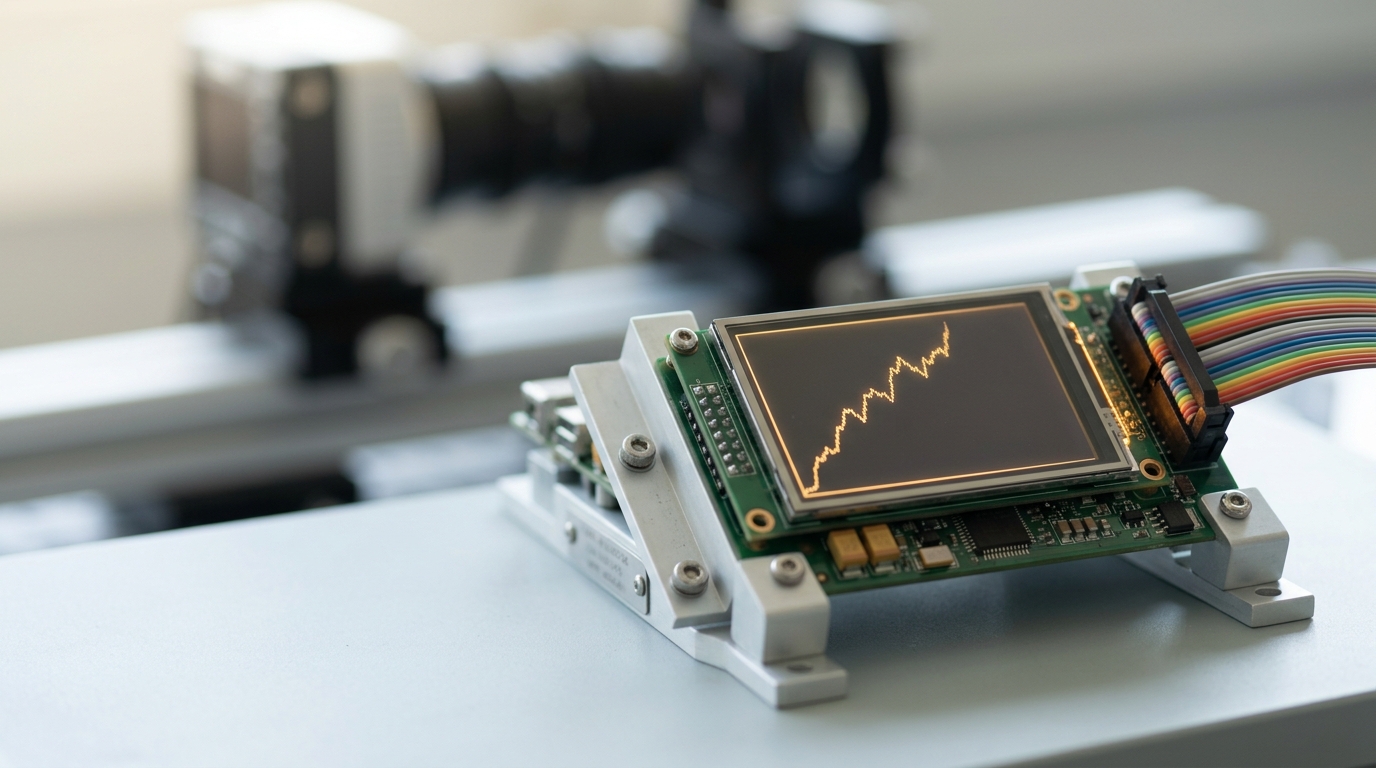
Its most consequential recent extension is the thermodynamic uncertainty relation, which states that in a nonequilibrium steady state, the precision of any time-integrated current — the number of steps a molecular motor takes, the number of substrate molecules an enzyme turns over — is bounded below by the total entropy production: a more precise current costs more dissipation, with no exceptions permitted below the bound [7]. A related result shows that this trade-off extends beyond the near-equilibrium, small-fluctuation regime where it was first derived, constraining the large-deviation function of steady-state currents even arbitrarily far from equilibrium [8]. This connects stochastic thermodynamics directly to large-deviation theory, discussed next, rather than keeping the two frameworks in separate silos.
What this class of methods is good for: universal precision-versus-dissipation trade-offs and trajectory-resolved entropy-production accounting for systems continuously coupled to a bath, whether or not they have a well-defined start and end state. It applies to steady states, not only finite-duration protocols, which fluctuation theorems in their basic form do not directly address. What it is not: a method for computing the probability of a specific rare event far in a distribution’s tail — the uncertainty relation gives a bound, not the tail probability itself — and its microscopic assumptions (a Markovian description at some coarse-grained level, a well-defined local heat bath at fixed temperature) do not hold automatically for every real system claimed to obey it; applying it to a system whose microscopic dynamics are not actually Markovian at the chosen level of coarse-graining is a documented failure mode, not a corner case.
Large-deviation theory: the probability of events too rare to sample directly
Large-deviation theory is older than either of the above and was not developed for thermodynamics specifically; it is a branch of probability theory concerned with the exponential decay rate of the probability of rare fluctuations of a sum of random variables, and it long predates its application to nonequilibrium physics [4]. Applied to a driven system, it asks a third kind of question: not “what is the equilibrium free energy” and not “what is the entropy production of this one trajectory,” but “how likely is it that the time-averaged current, or the total entropy production, over a long observation window takes an unusually large or small value, and at what exponential rate does that probability vanish as the observation window grows.”
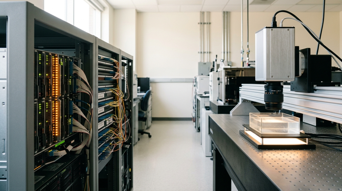
Answering that question analytically is hard for anything but the simplest models, which is why large-deviation theory in practice is inseparable from biased-sampling computational methods — cloning and splitting algorithms that steer an ensemble of simulated trajectories toward the rare event of interest rather than waiting for it to occur by chance in an unbiased simulation. This is the sense in which large-deviation theory is a computational and theoretical toolkit for a problem that direct trajectory recording cannot solve by brute force: the rare event of interest may be astronomically unlikely to show up in any dataset of directly recorded trajectories, however large.
What this class of methods is good for: the tails of the distribution — anomalously large currents, anomalously low entropy production, first-passage statistics for rare transitions — in systems where the object of interest is specifically the exponentially unlikely fluctuation, not the typical behavior. What it is not: an experimental measurement technique. Large-deviation results are almost always obtained from a model and a sampling algorithm rather than read directly off recorded data, because the events in question are, by construction, too rare to observe directly in finite recordings; connecting a large-deviation rate function back to a specific laboratory measurement typically requires an intermediate modeling step that fluctuation-theorem methods, which work directly from recorded trajectories, do not need.
The same three questions, asked of active matter and biological networks
The three frameworks do not stay confined to single-molecule biophysics; the harder and more interesting comparison is what happens when they are pointed at systems with no external experimenter choosing a forward and reverse protocol at all — active matter and living networks, where the driving is internal and continuous.
Active-matter systems — self-propelled colloidal particles, bacterial suspensions, cytoskeletal networks — are driven out of equilibrium by continuous internal energy consumption rather than a controlled external protocol, and this changes which framework is applicable. There is no clean forward-and-reverse pair of protocols to define a Crooks relation against in a self-propelled particle bath; the natural language is the entropy-production rate of stochastic thermodynamics or its steady-state large-deviation statistics. A study of interacting self-propelled particles found that for short but finite persistence time, the entropy-production rate can become small even though the system is manifestly out of equilibrium, showing that “distance from equilibrium” and “self-propulsion strength” are not the same axis and that entropy production must be computed rather than assumed from the presence of activity alone [9].
The problem sharpens further under coarse-graining. Real biological measurements rarely have access to every microscopic degree of freedom; they observe a handful of mesoscopic coordinates — the shape of a flagellum, the position of a bead attached to a cellular structure — and must infer whether the underlying process is out of equilibrium from that reduced view alone. Video microscopy combined with statistical inference has been used to detect broken detailed balance directly from recorded mesoscopic trajectories in beating flagella and primary cilia, without needing a microscopic model of the full molecular machinery driving them [10]. This is a genuinely different exercise from either fluctuation-theorem inference or large-deviation sampling: it is inference of irreversibility from a coarse-grained, partially observed system, and the central open difficulty is that coarse-graining can hide or manufacture apparent irreversibility depending on which coordinates are kept and which are averaged out — a caveat the original study itself treats carefully rather than overstating.
Reading the three frameworks against each other
Laid side by side on comparable dimensions, the picture is one of complementary reach rather than competition. Fluctuation theorems require a well-defined initial and final state and repeated trajectories with recorded work, and in exchange deliver an equilibrium quantity from nonequilibrium data — their proof of concept is the RNA-pulling experiments cited above. Stochastic thermodynamics’ entropy-production framework requires a Markovian description at some chosen coarse-graining level and delivers trajectory-resolved dissipation accounting and universal precision bounds that hold in steady states as well as driven protocols. Large-deviation theory requires either an analytically tractable model or a biased-sampling simulation and delivers the probability, and exponential decay rate, of fluctuations that are too rare to catch directly — at the cost of being, in practice, a computational rather than a directly experimental method.
None of the three subsumes the others, and the current research frontier is precisely in the overlaps: the thermodynamic uncertainty relation is a bridge result connecting stochastic thermodynamics’ entropy production to large-deviation statistics of currents [8]; active matter is a natural stress test for whether entropy-production language transfers cleanly to internally driven systems [9]; and mesoscopic biological inference is where the practical limits of coarse-graining are actually being worked out on real, imperfect data [10].
Where this plausibly goes next, and how to tell if it hasn’t
Over roughly the next five to eight years, the most likely direction of travel is toward hybrid inference pipelines that combine trajectory-level entropy-production estimators with biased-sampling large-deviation methods to extract rare-event statistics directly from partially observed, coarse-grained experimental data, rather than from idealized full-information models. This is a scenario, not a settled prediction: it assumes continued improvement in high-speed tracking hardware and continued interest from the biological-physics community in applying these tools to living systems rather than only to single-molecule benches. Observable indicators that this direction is succeeding would include entropy-production or uncertainty-relation estimators being applied directly to multi-particle active-matter video data with quantified error bars, and being cross- checked against independently derived large-deviation rate functions on the same dataset. The scenario would be disconfirmed, or at least substantially delayed, if coarse-graining-induced estimation bias — the concern already flagged in mesoscopic detailed-balance studies — turns out to be too severe to correct for on real biological data, forcing the field back toward idealized, fully observed model systems for the foreseeable future.
A note on notation, and where equations earn their place
Because these three frameworks share vocabulary, it is worth being explicit about the one place where a formal expression clarifies rather than decorates the comparison: the Jarzynski equality itself. Written compactly, it states
where
The discipline the comparison enforces
The value of holding these three frameworks apart is not pedantry. A result obtained under the fluctuation-theorem framework licenses a claim about an equilibrium free-energy difference recovered from a specific nonequilibrium protocol; it does not license a claim about the entropy-production rate of an unrelated steady-state system, and it certainly does not license a claim about the probability of a specific rare fluctuation in that system’s tail. Each framework was built to answer one question well, tested against a specific and limited class of experiments, and left with its own open failure modes — coarse-graining bias for entropy-production inference, sampling cost for large-deviation estimation, repeatability requirements for fluctuation-theorem protocols. Comparing the frameworks on these terms, rather than ranking them, is what the current state of nonequilibrium statistical physics actually supports.