Ask three Earth scientists how much the planet has warmed and you will get, in a sense, three different instruments answering three different questions. A paleoclimatologist will point to an ice core and describe a range of temperature swings measured in kelvin over hundreds of thousands of years, inferred from the ratio of oxygen isotopes trapped in ancient snow. An observational climatologist will point to a network of thermometers, buoys and satellites and quote a trend since 1880, expressed in tenths of a degree per decade, with an explicit confidence interval. A modeler will point to an ensemble of simulations run on a supercomputer and describe a distribution of possible futures under a given emissions pathway, none of which is a measurement of anything that has happened yet.
None of these three is a cruder or more advanced version of the other two. They are structurally different approaches to the same physical system, and each is suited to a different part of the problem. Paleoclimate proxy reconstruction is the only way to see the climate system’s behavior over spans longer than living instruments, at the cost of resolution and unavoidable interpretive assumptions in translating a physical proxy into a temperature or a gas concentration. Direct instrumental and satellite observation gives high-resolution, high-precision data, but only for the last several decades to roughly a century and a half, and even that record has to be corrected for changing instruments and observing practices. General circulation model (GCM) simulation is the only way to test cause-and-effect hypotheses about the future or about counterfactual pasts, because a model, unlike a proxy or a thermometer, can be run with one variable held fixed while others change — but a model is not a record of anything that occurred, it is a numerical solution to approximated physics, and its output is only as good as its representation of processes it cannot itself observe.
This article compares the three approaches directly, on the dimensions that actually distinguish them — temporal coverage, spatial and temporal resolution, and the specific sources of uncertainty each carries — across six recurring problems in climate science: radiative forcing, the carbon cycle, ocean heat content and circulation, ice mass balance, extreme-event attribution, and future projection. The goal is not to declare a winner. It is to show what each approach can and cannot tell you, so that a number quoted from one of them is read as answering the question that method actually asks.
Three approaches, one system
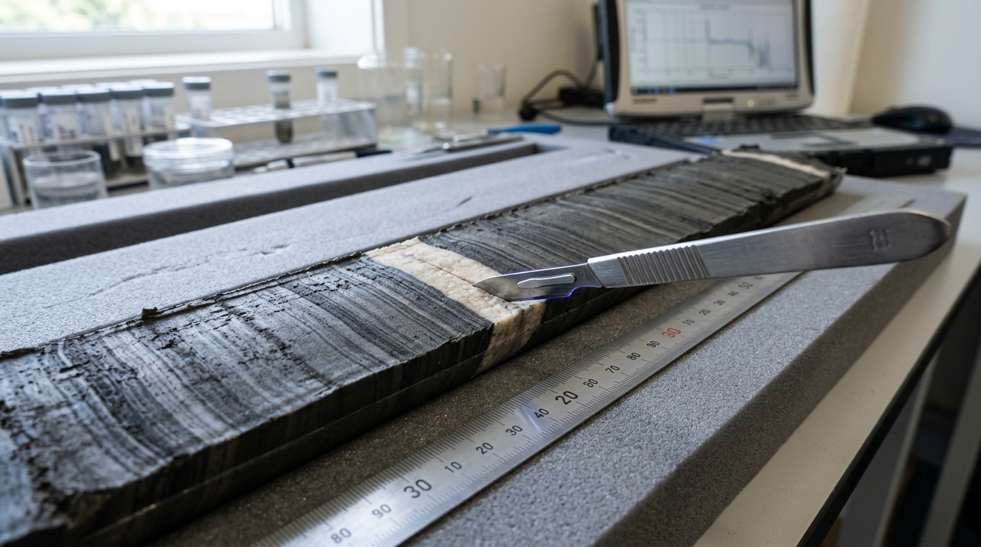
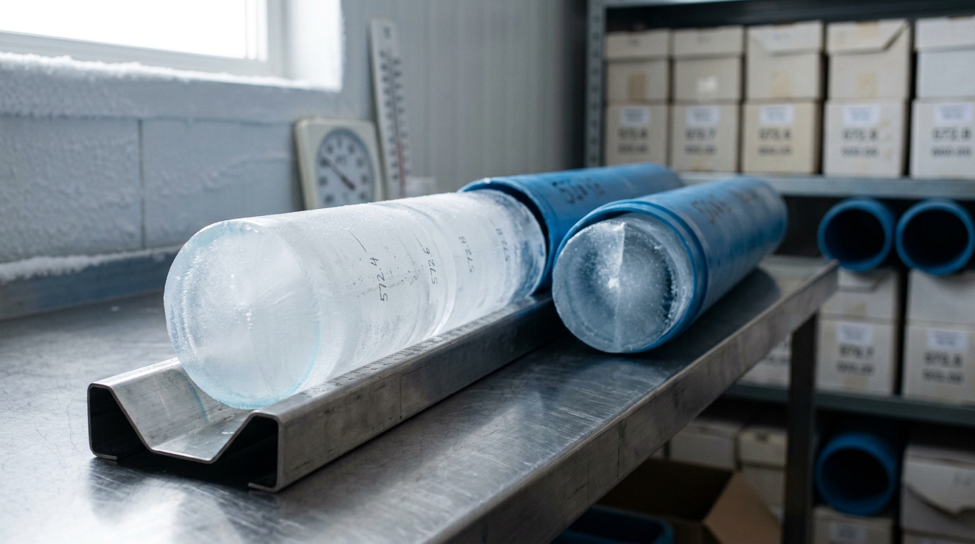
Paleoclimate proxy reconstruction infers past climate conditions from physical, chemical or biological traces left in natural archives: air bubbles and dust trapped in polar ice, the isotopic composition of shells in ocean sediment, tree-ring widths, coral growth bands, cave formations. The archive itself was not built to record climate — the inference runs backward from a physical or chemical signal to an environmental cause, using calibrations built from the modern instrumental period or from independent physical theory. The EPICA Dome C core from East Antarctica reaches roughly 800,000 years into the past through a physical column of ice roughly 3.2 kilometers deep, and NOAA’s paleoclimatology archive holds records like it from polar and mountain ice caps worldwide, describing the proxies typically used as “oxygen isotopes, methane concentrations, dust content, and many other parameters” drawn from ice recovered at sites from Greenland’s GISP2 dome onward [5]. Marine sediment cores extend the same logic further back, at coarser time resolution, using the ratio of oxygen isotopes in the shells of bottom-dwelling foraminifera as a joint proxy for ice volume and deep-ocean temperature.
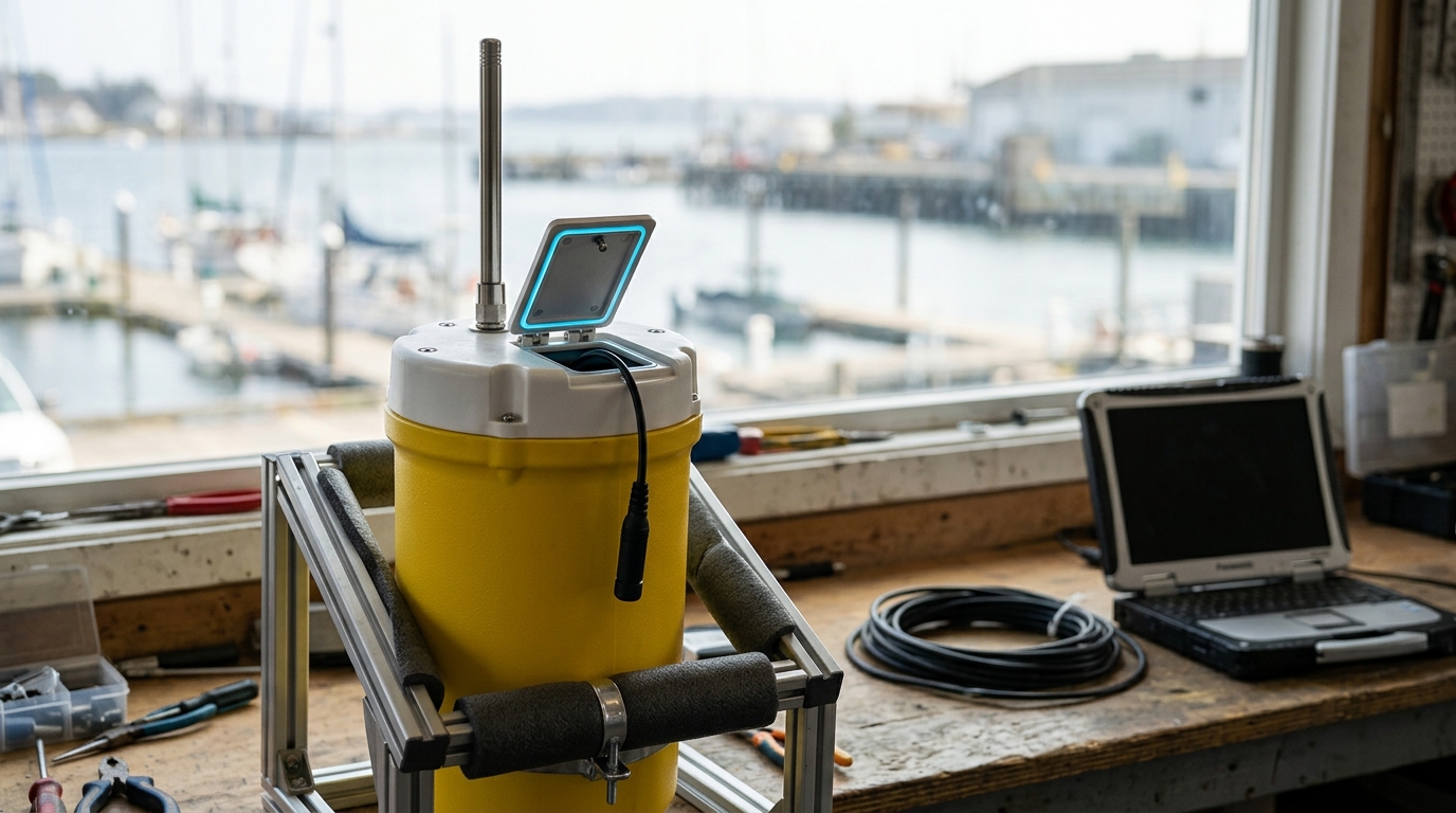
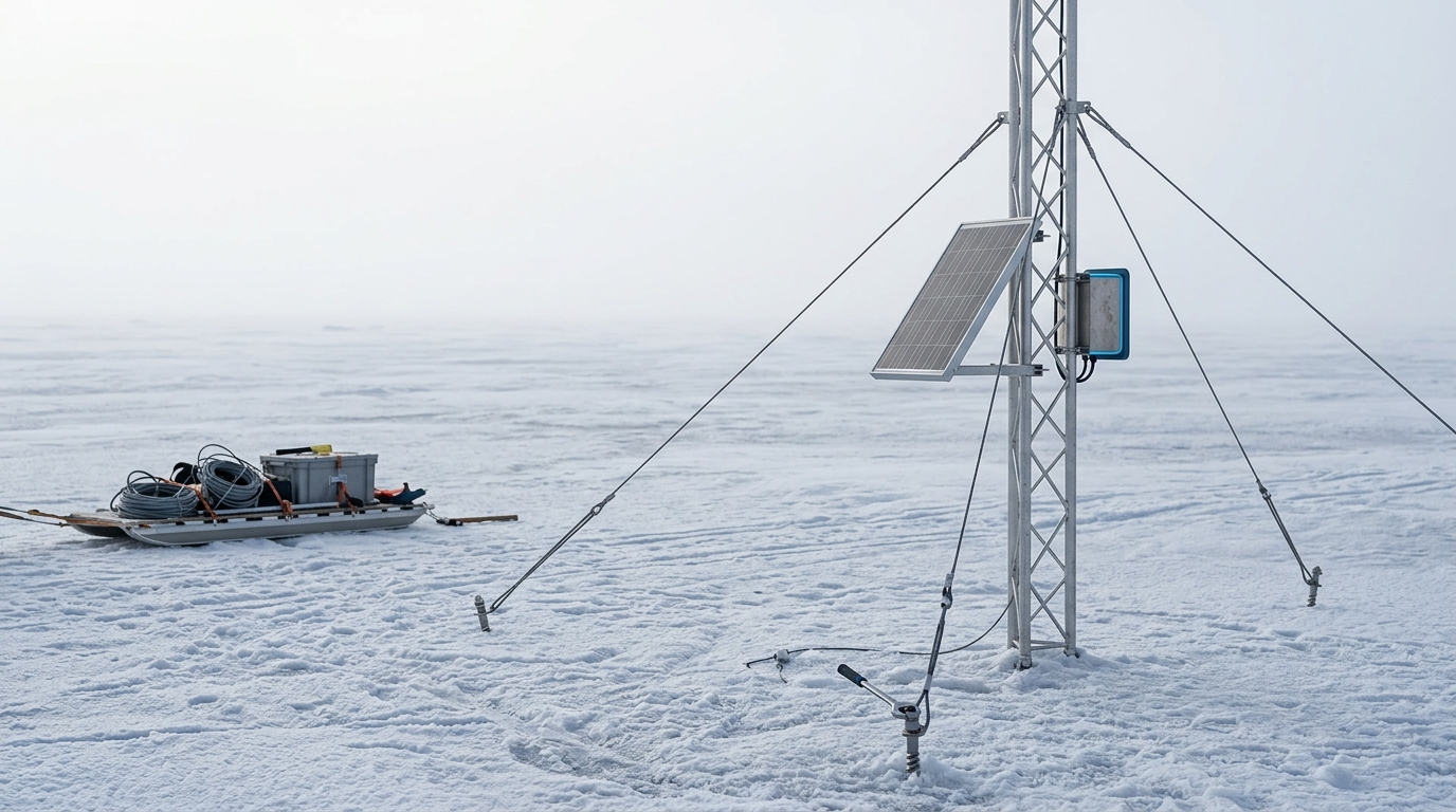
Direct instrumental and satellite observation measures the present climate system with physical sensors built for that purpose: thermometers, barometers, tide gauges, weather balloons, moored ocean buoys, satellite radiometers and gravimeters, and — since the early 2000s — a global fleet of autonomous profiling floats. NASA’s GISTEMP analysis combines land meteorological station records (NOAA’s GHCN) with sea-surface temperature data (ERSST) into a single global surface temperature index, a methodology whose modern form NASA traces to work “defined in the late 1970s by James Hansen” and which is updated monthly against a 1951–1980 baseline [8]. The Argo program has, since the early 2000s, maintained an international fleet of robotic floats that “drift with the ocean currents and move up and down between the surface and a mid-water level,” measuring temperature and salinity through the top 2,000 meters of the global ocean [3]. Tropical mooring networks — TAO in the Pacific, PIRATA in the Atlantic, RAMA in the Indian Ocean, together forming NOAA’s Global Tropical Moored Buoy Array — add fixed-point, high-frequency measurements of the upper ocean and overlying atmosphere at specific locations, useful for capturing short-lived events like El Niño development that a slower-moving float network can under-sample [6]. Satellite programs add nearly continuous global coverage: NASA notes that ice-sheet mass loss is tracked through gravity measurements from the GRACE mission (2002–2017) and its successor GRACE Follow-On, finding “Antarctica is losing ice mass at an average rate of about 135 billion tons per year, and Greenland is losing about 264 billion tons per year” [2].
General circulation models solve discretized versions of the physical equations governing fluid motion, radiative transfer, and thermodynamics on a three-dimensional grid spanning the atmosphere, ocean, land surface and sea ice, coupling those components so that heat, moisture and momentum move between them over a simulated time series. The Geophysical Fluid Dynamics Laboratory, which built what it describes as the first coupled ocean-atmosphere general circulation climate model beginning in the 1960s, still develops and runs GCMs to simulate “the atmosphere, ocean, land surface, and sea ice” and their interactions, at time and space resolutions set by available computing capacity rather than by what a proxy or an instrument happened to preserve [4]. The current international coordination for this work is the Coupled Model Intercomparison Project, now in its sixth phase (CMIP6), which the World Climate Research Programme describes as having “become essential to the Intergovernmental Panel on Climate Change (IPCC) and other international and national climate assessments,” organized around a common core of experiments — the DECK and CMIP historical simulations — plus 23 endorsed sub-projects addressing specific scientific questions [7]. A model run is not an observation; it is a hypothesis about physical mechanism, expressed as an equation system and then executed. Its output can be compared against the historical instrumental and paleoclimate record as a test of whether the mechanism is adequate, and it can be run forward under assumed future forcing as a scenario projection — the latter being, definitionally, not a fact about the world.
Radiative forcing: three different evidentiary paths to one number
Radiative forcing — the net change in the balance between incoming and outgoing radiation caused by greenhouse gases, aerosols and other perturbations — is estimated by all three approaches, but from different evidence.
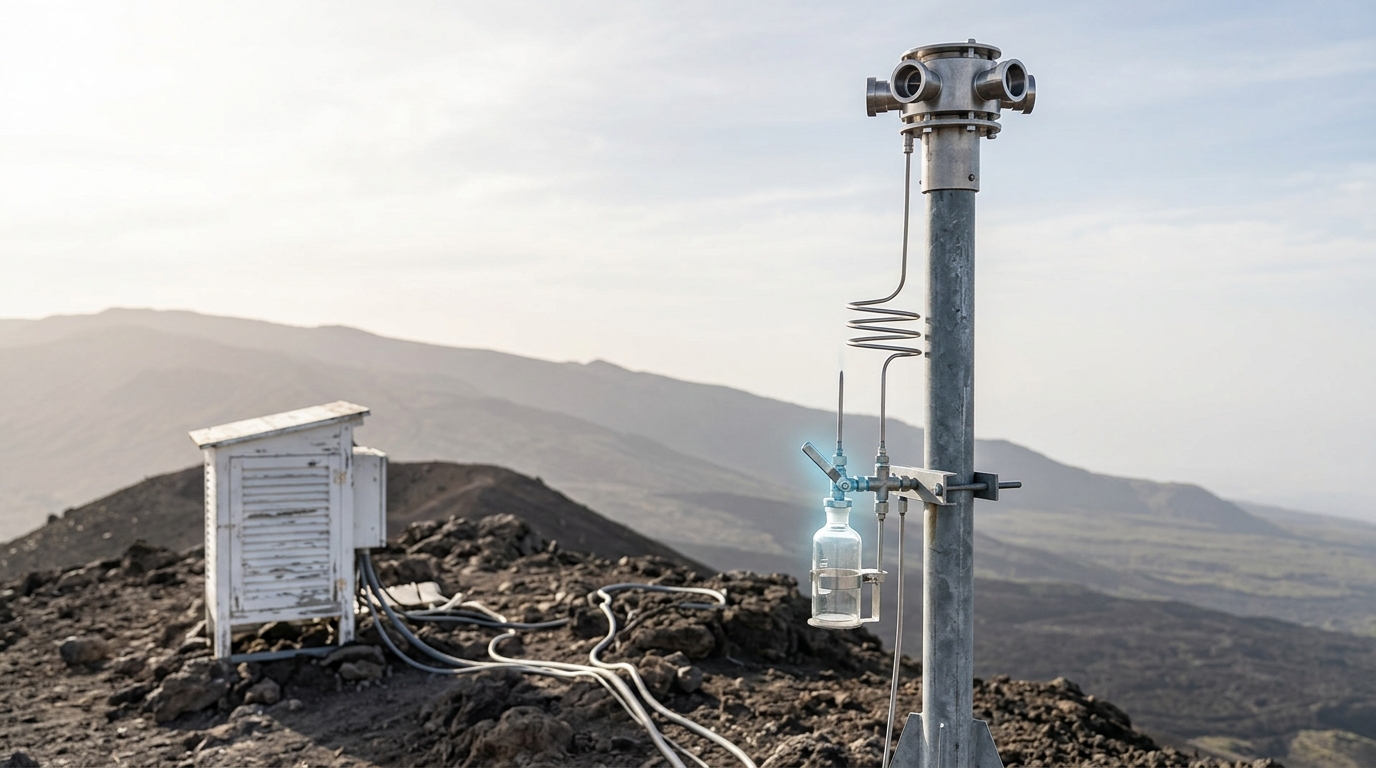
The instrumental path is the most direct: atmospheric composition is measured, not inferred, at monitoring stations such as Mauna Loa Observatory, where the July 2026 monthly average stood at 429.12 parts per million, part of what NOAA describes as “the longest record of direct measurements of CO2 in the atmosphere,” begun by Charles David Keeling in 1958 with NOAA running an independent parallel record since 1974 [1]. From concentration, radiative forcing follows from established infrared absorption physics — this is analysis built on a physical law, not a proxy inference, though the translation from a well-mixed global gas concentration to a spatially and temporally resolved forcing still carries modeling assumptions about atmospheric structure.
The paleoclimate path reconstructs forcing indirectly: gas concentrations trapped in ice-core air bubbles give a direct paleo-atmosphere sample rather than a proxy in the strict sense, but converting the ice’s isotopic composition into a paleotemperature requires an assumed physical relationship between isotope fractionation and past temperature, calibrated against modern conditions and therefore carrying its own systematic uncertainty that does not shrink with more ice — it is bounded by how well the calibration itself is known.
The modeled path treats forcing as an input a GCM is told to apply, then tests whether the physics inside the model reproduces the observed or paleo-reconstructed temperature response to that forcing. This is where the CMIP framework becomes load-bearing: it is explicitly organized to test, among other things, “how does the Earth system respond to forcing” as a scientific question, using the historical simulation experiments as a check against the instrumental record rather than as an independent estimate of the forcing itself [7].
The three paths converge on the same physical picture, but for genuinely different reasons: measured composition plus known physics; inferred paleo-composition plus a calibrated proxy relationship; and modeled response, validated against the other two. Treating a modeled sensitivity number as though it had the same evidentiary status as a Mauna Loa flask measurement, or treating an isotope-derived paleotemperature as though it had instrumental-grade resolution, both misdescribe the method.
The carbon cycle: continuous flask record versus discrete ancient samples
This mass-balance identity — the rate of change of atmospheric carbon equals emissions minus net ocean and land uptake — is the same equation whether it is applied to this decade or to a glacial cycle 400,000 years ago, but the three approaches populate its terms with evidence of very different character.
The instrumental record measures
The paleoclimate record measures
GCMs, when run with an interactive carbon cycle rather than a prescribed concentration, attempt to simulate
Oceans: depth-resolved present versus centuries-old deep signal
The ocean absorbs the large majority of the additional heat retained by the climate system, and here the three approaches address genuinely different volumes and timescales of the ocean rather than the same signal at different resolutions.
Direct measurement of the upper ocean is now dense and depth-resolved thanks to the Argo float network, which profiles temperature and salinity through the top 2,000 meters on a roughly ten-day repeat cycle per float, across a globally distributed array — a design built specifically to remove the sparse, ship-track sampling bias of the pre-Argo era [3]. Fixed tropical moorings such as TAO, PIRATA and RAMA add continuous, high-frequency time series at specific points, which is what allows short-duration, fast-developing phenomena like an El Niño onset to be tracked in near real time in a way a slower-cycling float array cannot resolve as sharply [6]. Neither network has been deployed long enough, however, to directly measure deep-ocean (below 2,000 meters) heat content trends with the same confidence, and neither has direct coverage before the early-to-mid twentieth century for surface data, or the early 2000s for the Argo-depth-resolved record.
Paleoceanographic proxies — benthic foraminiferal oxygen isotopes in sediment cores chief among them — are the primary source of information about ocean state on timescales of thousands to millions of years, including deep-ocean temperature and global ice volume jointly, because the isotopic signal mixes both effects and requires independent assumptions to separate them. This is a genuine resolution trade: sediment cores see far deeper time than any thermometer record, but at temporal resolution measured in centuries to millennia per sample rather than days, and with an unavoidable convolution of two physical signals (temperature and ice volume) that must be disentangled analytically rather than measured apart.
GCMs with coupled ocean components are the only approach that can simulate ocean heat uptake and large-scale circulation — including features like the Atlantic overturning circulation — as a continuous, three-dimensional, time-evolving field for periods where no observational network existed at all, past or future. That capability is also the model’s principal liability here: deep-ocean circulation operates on multi-century timescales, so a model’s representation of it is validated against a comparatively short instrumental record and a coarser paleoceanographic one, leaving open exactly the low-frequency behavior that matters most for centuries-ahead projection.
Ice mass balance and sea level: satellite gravimetry versus surface mass-balance stakes
Direct satellite observation of ice-sheet mass balance is a case where the instrumental approach has essentially no paleoclimate or early-instrumental analogue at comparable precision. NASA reports that GRACE (2002–2017) and GRACE Follow-On (since 2018) gravimetry find Antarctica losing about 135 billion tons of ice per year and Greenland about 264 billion tons per year, contributing roughly 0.4 and 0.8 millimeters per year respectively to global sea-level rise over the 2002–2025 span [2]. This is a genuinely new observational capability: nothing before satellite gravimetry could measure whole-ice-sheet mass change directly, as opposed to inferring it from surface elevation surveys or mass-balance stake networks at a limited number of points.
Paleoclimate reconstruction supplies the only evidence for how ice sheets have behaved across full glacial-interglacial cycles — repeated advances and retreats over hundreds of thousands of years recorded in the same ice-core and sediment-core archives already discussed — which is essential context for judging whether current rates of loss are within or outside the range of past natural variability, but it cannot resolve annual-to-decadal rates with anything like GRACE’s precision; a proxy record averaged over centuries structurally cannot show a rate change occurring over two decades.
GCMs coupled to ice-sheet dynamics models are used to project how mass balance will evolve under future warming, translating physical processes — surface melt, ice-shelf basal melting, ice-dynamic discharge — into a forward estimate. Ice-sheet dynamics remain one of the more poorly constrained components of Earth-system models precisely because the observational record used to validate them (the satellite era) is short relative to the processes involved, such as multi-century ice-shelf collapse dynamics.
Extreme-event attribution: where all three approaches meet and none is sufficient alone
Attributing a specific extreme event — a heat wave, a flood, a drought — to human-caused climate change illustrates why the three approaches are complementary rather than substitutable, because attribution science characteristically needs all three inputs at once. The instrumental record establishes that the observed event was statistically unusual against the modern baseline. Paleoclimate and long instrumental reconstructions establish the event’s rarity against a longer natural-variability baseline than the instrumental record alone can provide, which matters because a “record-breaking” event assessed only against a 50-to-150-year instrumental baseline may not be so unusual against a longer natural range. GCM experiments then supply the counterfactual: running large ensembles of the same model under estimated pre-industrial versus current forcing to estimate how much more likely, or more intense, the same event class became — a question no observational record, however long, can answer directly, because there is only one observed history and no observed counterfactual.
Each input carries a distinct uncertainty. The instrumental classification depends on how “unusual” is defined and over what baseline period. The long-baseline context from paleoclimate depends on how comparable a proxy-inferred regional extreme actually is to the modern, precisely defined event. The model-based counterfactual depends on how well the GCM’s regional climate — often at resolutions of 100 kilometers or coarser in the CMIP6 generation, refined further only in dedicated regional or storyline studies — captures the physical processes that produced the specific event, which for phenomena like localized convective storms can be a real limitation.
Where the disagreements actually sit
It is worth being explicit about where these three approaches genuinely disagree today, rather than simply agreeing on a shared physical picture at different resolutions.
Model spread in equilibrium climate sensitivity — the long-term warming expected per doubling of atmospheric carbon dioxide — has narrowed across CMIP generations but has not converged to a single value; different models retain different cloud-feedback representations, and that spread is a genuine, currently unresolved scientific disagreement about atmospheric physics, not a data gap that more observation alone will close on any short timescale, because the relevant feedback processes operate on timescales instruments have not yet fully sampled.
Deep-ocean and ice-sheet response timescales are where paleoclimate evidence and model projection are hardest to reconcile directly, because the paleo record shows these systems can change abruptly after long apparent stability — a nonlinearity that is difficult for a model tuned against a comparatively quiescent instrumental period to reproduce with confidence, and difficult for a proxy record to date and resolve at the same abruptness scale it may actually have occurred.
Regional precipitation projection shows genuine, substantial inter-model disagreement even in sign, in some regions, for reasons tied to how convection and monsoon dynamics are parameterized rather than resolved from first principles at typical GCM grid spacing — a limitation of the modeling approach specifically, not resolvable by better paleoclimate or instrumental data on the region in question, because the disagreement is about mechanism representation rather than about what happened.
What each approach cannot tell you
It is as important to state the limits plainly as the strengths.
Paleoclimate reconstruction cannot give you a rate of current, ongoing change with instrumental precision, cannot give you global coverage — proxy archives exist where nature happened to preserve them, not where scientific coverage is most needed — and requires a calibration to convert a physical proxy into an environmental variable, a step that carries irreducible uncertainty distinct from measurement noise.
Direct instrumental and satellite observation cannot see further back than the instrument existed, cannot by itself establish cause (a measured trend is a fact, not an attribution), and even within the instrumental era carries known inhomogeneities — station relocations, changing observation times, sensor replacement — that have to be statistically corrected for, a process that is itself a modeling exercise layered on top of the raw measurement.
GCM simulation cannot observe anything; every model output is conditional on the physics coded into it and the scenario assumptions fed into it, and a projection’s plausibility rests entirely on how well the model reproduces the instrumental and paleoclimate record it is checked against — which is exactly why the other two approaches remain indispensable rather than superseded by increasing computational power.
A forward-looking claim, stated as a scenario rather than a fact
Scenario, not prediction of fact: if current trends in computational capacity and observational coverage continue over the next decade, GCM horizontal resolution in the routine CMIP-class ensemble is likely to improve enough to explicitly resolve, rather than parameterize, some categories of organized convection in a growing fraction of participating models, which would narrow (not eliminate) inter-model spread in regional precipitation projection specifically. This is conditional on sustained computing investment and on no methodological pivot away from the CMIP coordination framework; the observable indicator to check in ten years is whether the CMIP7-or-successor generation’s stated horizontal grid spacing for standard-tier models has fallen meaningfully below the roughly 100-kilometer class typical of CMIP6, and whether published inter-model precipitation spread in convection-affected regions has measurably narrowed as a direct consequence rather than for unrelated reasons. If grid spacing does not fall and precipitation spread does not narrow specifically in the regions where convective parameterization was the identified cause, the scenario is disconfirmed.
Reading a climate number correctly
The practical upshot for a reader encountering a climate statistic is to ask, before anything else, which of the three approaches produced it. A number from an ice core is a proxy-calibrated inference over a long, low-resolution timescale. A number from a satellite or a buoy network is a direct, high-resolution measurement over a short timescale, itself subject to correction and known coverage gaps. A number from a model run is a conditional projection, valid only to the extent the model’s physics has been validated against the other two records, and never itself a fact about the world it describes. Climate science is convincing not because any one of these three approaches is decisive on its own, but because the picture they jointly constrain — a warming, energy-imbalanced planet with rising atmospheric carbon dioxide, shrinking ice sheets and shifting extremes — holds up under three structurally independent kinds of scrutiny at once.