Three claims that are usually stated, rarely shown
“Greenhouse gases are warming the planet,” “the ocean is absorbing most of the excess heat and a large share of the excess carbon,” and “climate models project a range of futures” are three of the most repeated sentences in public science writing. They are also three of the least explained. Each is a shorthand for an actual measurement chain: an instrument, a calibration standard, a network of stations or floats or satellites, a reconciliation procedure, and a stated uncertainty. This article opens a series on Earth systems and climate dynamics by building those chains from the ground up — what is measured, how, by whom, and what is not yet resolved.
The scope here is deliberately narrow and mechanical. It covers how radiative forcing from greenhouse gases is measured and attributed to specific gases, how the global carbon cycle’s ocean, land, and atmospheric fluxes are quantified and reconciled against each other, and what a climate-model ensemble actually represents — including where its uncertainty comes from and what that uncertainty does and does not license someone to say. Sea level, ice, and extreme-event attribution appear as downstream consequences of the same forcing and flux accounting, not as separate topics.
Radiative forcing is measured, not merely calculated from emissions
Radiative forcing is the change in the balance between incoming solar energy and outgoing infrared energy at the top of the atmosphere (or, in some formulations, at the tropopause) caused by a change in atmospheric composition or other climate driver, expressed in watts per square metre. It is tempting to treat forcing as something computed purely from an emissions inventory run through a formula. It is not. Forcing rests on three independently measured layers, each with its own instrumentation.
The first layer is atmospheric concentration itself. The longest continuous record is the Mauna Loa Observatory carbon dioxide series, begun by Charles David Keeling in March 1958 and continued today by NOAA’s Global Monitoring Laboratory alongside the Scripps Institution of Oceanography’s parallel record [2]. Air is drawn from an intake mast, dried, and passed through a nondispersive infrared analyzer that measures absorption at a wavelength band where CO2 is strongly absorbing; the instrument is calibrated against a suite of reference gas mixtures with concentrations traceable to a primary standard, and the result is a monthly mean with a documented measurement uncertainty. As of mid-2026 that record shows atmospheric CO2 above 429 parts per million, up from a pre-industrial baseline near 280 ppm — a fact drawn directly from the instrument record, not an estimate [2].
The second layer is the translation from concentration to forcing. This is where the nondispersive infrared measurement principle becomes physically central rather than incidental: a gas’s radiative forcing depends on how strongly and at which wavelengths it absorbs and re-emits infrared radiation, which is exactly the property the analyzer exploits to detect it in the first place. Radiative transfer calculations, validated against satellite spectral measurements of outgoing longwave radiation, convert a measured concentration change into a forcing value in watts per square metre. NOAA’s Annual Greenhouse Gas Index compiles this translation for the long-lived, well-mixed greenhouse gases — carbon dioxide, methane, nitrous oxide, and a set of halogenated compounds — using measured concentrations from a global flask-sampling and continuous-monitoring network [1]. The AGGI reports that radiative forcing from these gases was 54 percent higher in 2024 than in 1990, with carbon dioxide responsible for roughly 81 percent of that increase [1]. That is an attributed breakdown by gas, built from measured concentrations and known absorption physics — not an assumption that all warming is CO2’s alone.
The third layer is the direct check on the whole chain: does measured forcing show up as a measured energy imbalance at the top of the atmosphere and inside the climate system? This is where the ocean enters as an instrument rather than a passive backdrop, addressed below.
is the standard simplified radiative-forcing relation for CO2, where

None of this is a single number handed down by authority. It is a chain of measurements: flask and continuous concentration data, calibrated against primary standards, converted through radiative transfer physics validated against satellite spectral observations, cross-checked against a measured planetary energy imbalance. Each link carries its own documented uncertainty, and the uncertainty is generally smallest for concentration measurement and largest for aerosol forcing, which partially offsets greenhouse-gas forcing and remains the least well-constrained term in the global energy budget.
The carbon cycle is reconciled, not assumed
The global carbon cycle question that matters operationally is simple to state and hard to answer with confidence: of the carbon dioxide emitted by fossil fuel combustion and land-use change each year, how much stays in the atmosphere, how much is taken up by the ocean, and how much is taken up by land ecosystems? The Global Carbon Project’s annual Global Carbon Budget answers this by combining several independent observing systems and reconciling them against each other rather than trusting any single method [3].
Fossil emissions are estimated from energy-consumption statistics, cement production data, and national inventories — an activity-based accounting method, not a direct atmospheric measurement. Land-use change emissions are estimated from bookkeeping models of deforestation, afforestation, and land management, informed by satellite land-cover data. The atmospheric growth rate — how much CO2 concentration actually increases each year — is measured directly from the same flask and continuous networks that underlie the AGGI. Ocean uptake is estimated from a combination of ocean biogeochemistry models, surface ocean CO2 partial-pressure measurements taken from research vessels and autonomous platforms, and inventories of dissolved inorganic carbon. Land uptake — the net effect of photosynthesis, respiration, and disturbance across all terrestrial ecosystems — is the least directly observable term and is typically estimated as a residual: total emissions minus atmospheric growth minus ocean uptake, cross-checked where possible against independent terrestrial carbon-cycle models and forest-inventory data.
The 2023 Global Carbon Budget reports fossil CO2 emissions of 9.9 ± 0.5 gigatonnes of carbon per year, with global emissions still increasing through the assessed period, and it publishes uncertainty ranges on every flux term rather than a single reconciled figure [3]. That the land sink is calculated partly by subtraction is a genuine limitation, not a hidden one: it means errors in any of the other three terms propagate directly into the land-uptake estimate, and it is why the Global Carbon Project’s yearly assessment includes an explicit budget imbalance term — the amount by which independent estimates of the four fluxes fail to sum to zero. Reporting that imbalance, rather than forcing the books to close, is the more scientifically honest choice, and it is a direct, verifiable indicator of how much slack remains in the accounting.
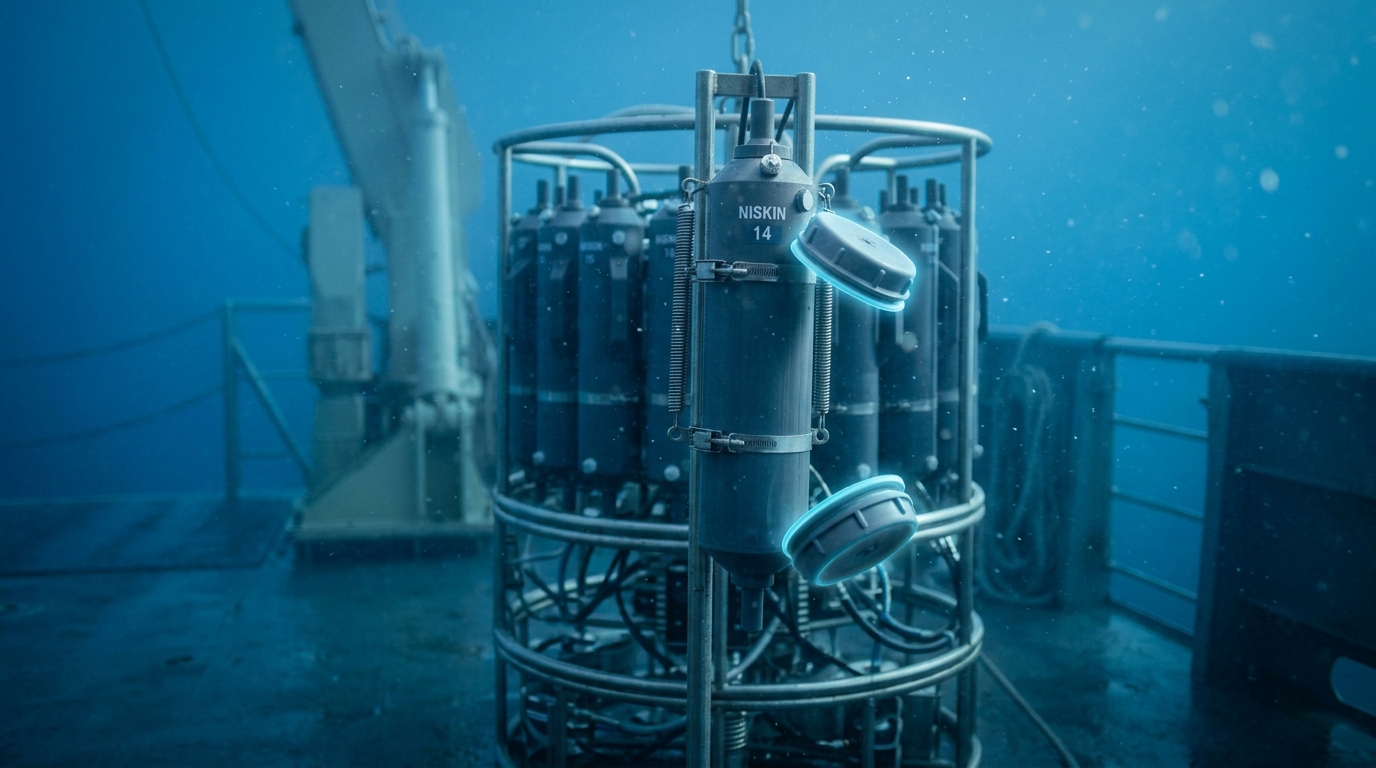
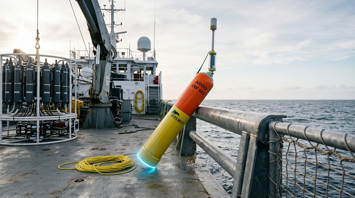
The ocean’s role deserves its own emphasis because it is doing two jobs simultaneously: absorbing roughly a quarter of annual anthropogenic CO2 emissions, and absorbing more than 90 percent of the additional heat trapped by the enhanced greenhouse effect [3] [5]. The instrument that makes the second figure measurable is the global Argo float array — several thousand autonomous profiling floats that drift with ocean currents, periodically dive to roughly 2,000 metres, and rise back to the surface measuring temperature and salinity along the way before transmitting data by satellite [6]. NOAA’s National Centers for Environmental Information compiles these profiles, along with historical ship-based measurements, into gridded ocean heat content fields updated quarterly, covering depths from the surface to 2,000 metres and extending back to 1955 [5]. Ocean heat content is arguably a cleaner diagnostic of the planet’s energy imbalance than surface air temperature, because the ocean’s heat capacity swamps transient atmospheric variability — a single El Niño or volcanic eruption barely dents a multi-decadal ocean heat content trend, whereas it visibly perturbs the surface temperature record.
What a climate-model ensemble actually is
A climate model is a numerical solution to the coupled equations governing atmospheric and oceanic fluid dynamics, radiative transfer, and a set of parameterized sub-grid processes — cloud formation, convection, sea ice dynamics, land-surface hydrology — that occur at scales finer than the model’s computational grid can resolve directly. No single run of such a model is “the forecast.” An ensemble is a set of runs that differ in initial conditions, in physical parameterization choices, or in both, executed to characterize the range of outcomes consistent with the same underlying physics and the same emissions scenario.
This structure separates two distinct sources of spread that are routinely conflated in public discussion. Internal variability is the spread produced by chaotic sensitivity to initial conditions — the same physics, run from slightly different starting points, producing different weather trajectories that only converge in their statistics over years to decades. Structural or parametric uncertainty is the spread produced by different models, or different parameter choices within one model, representing genuinely different assumptions about unresolved physical processes such as cloud feedback strength. A third source, scenario uncertainty, is not a model property at all — it is the range of possible future emissions trajectories, which depends on human decisions the models do not predict and are not designed to predict.
Conflating these three is the most common category error in popular treatments of climate projections. A statement like “models project 2.7 degrees of warming by 2100” is meaningless without specifying: under which emissions scenario, across which model ensemble, and whether the figure is a central estimate or a bound of a stated range. The IPCC’s assessment practice — synthesizing multiple independent model ensembles (the Coupled Model Intercomparison Project generations) alongside observational constraints — exists specifically to keep these sources of uncertainty distinct and to avoid presenting a chaotic weather-scale spread and a genuine physical disagreement about cloud feedbacks as though they were the same kind of uncertainty.
It is also worth stating plainly what an ensemble spread is not. It is not a confidence interval in the strict statistical sense, because model ensembles are not random samples from a well-defined population — they are “ensembles of opportunity,” built from whichever modeling centres submitted runs, with structural interdependencies between models that share code lineage or tuning targets. Treating the ensemble spread as a rigorous probability distribution overstates precision the ensemble was never designed to provide. What the spread does reliably show is the range of physically self-consistent outcomes current models can produce under stated assumptions, and where that range is narrow versus where it remains wide — global mean surface temperature trends are comparatively well constrained across models; regional precipitation change and cloud feedback strength remain comparatively poorly constrained.
Ice, sea level, and the observational chain that connects them
Two further observing systems close the loop between forcing and consequence. The Argo array and satellite altimetry jointly constrain sea level rise: NASA’s Sea Level Change Portal compiles satellite radar altimetry going back to 1993 together with tide-gauge records, reporting that the rate of global mean sea level rise has roughly doubled over the past three decades and that 2024 saw sea level rise faster than the multi-decadal trend alone would predict [7]. That acceleration is attributed, through the same kind of component-by-component accounting used in the carbon budget, to a combination of thermal expansion of ocean water (tracked through the same ocean heat content data used above) and mass loss from the Greenland and Antarctic ice sheets and mountain glaciers, tracked independently through satellite gravimetry and altimetry missions.
Sea ice extent is monitored separately and continuously by the National Snow and Ice Data Center, which compiles satellite passive-microwave imagery into a daily-updated Arctic and Antarctic sea ice record [8]. Sea ice extent is a useful complementary indicator precisely because it responds to regional atmospheric and oceanic circulation on top of the long-term forcing trend, so a single year’s anomaly is not, by itself, an attribution claim — it is one data point in a record whose trend is the actual signal of interest.
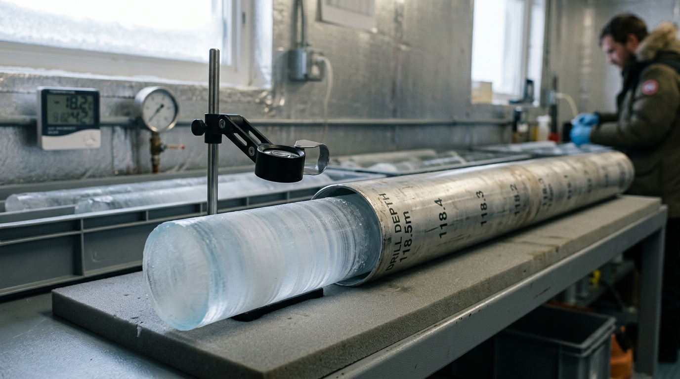
The instrumental record described so far extends back to the late 1950s at best for direct atmospheric CO2 measurement, and to the 1880s for a global surface temperature record built from meteorological stations, ships, and — more recently — satellite and ocean-based measurements combined by NASA’s Goddard Institute for Space Studies into a single global anomaly series relative to a 1951–1980 baseline [4]. That record shows the ten most recent years as the warmest in the series, with 2024 the single warmest year measured and 2025 statistically close behind it [4]. To go further back than direct instruments allow, paleoclimate archives — ice cores, ocean and lake sediment cores, corals, tree rings — extend the record over hundreds of thousands of years by preserving physical or chemical proxies for past temperature and atmospheric composition, most directly through air bubbles trapped in ice that constitute literal samples of ancient atmosphere. These archives are what make it possible to say the current CO2 concentration and its rate of increase are without precedent in a comparably long window, a claim that rests on physical samples rather than on modeling.
Monthly synthesis of all these observing systems is compiled by NOAA’s National Centers for Environmental Information into a routine monthly climate report combining global and national temperature, precipitation, and other indicators [10], and annually by the World Meteorological Organization’s State of the Global Climate report, which in recent years has documented what its authors describe as increasingly pronounced departures from historical baselines across temperature, ocean heat, sea level, and cryosphere indicators simultaneously [9]. These are institutional syntheses of the underlying measurement networks described above, not independent new measurements — their value is in cross-checking that the component records tell a consistent story.
Separating fact, attribution, scenario, and prediction
It is worth being explicit, at the end, about which kind of claim each part of this article makes, because the categories are routinely blurred in public discussion of climate science.
Fact, directly measured: atmospheric CO2 concentration and its trend [2]; global mean surface temperature anomaly and its trend [4]; ocean heat content and its trend to 2,000 metres [5]; sea level rise rate from satellite altimetry [7]; Arctic and Antarctic sea ice extent [8].
Analysis, built from measurements through a stated physical model: the translation of measured gas concentrations into radiative forcing values using radiative transfer physics [1]; the attribution of forcing increase by gas [1]; the partitioning of emitted carbon among atmosphere, ocean, and land sinks, including the explicit residual and imbalance terms [3].
Scenario, not prediction: any statement of the form “under a given emissions pathway, models project X degrees of warming.” The emissions pathway is a scenario choice representing possible human decisions, not a physical inevitability, and should always be stated alongside the number.
Genuine scientific uncertainty, not settled: the precise magnitude of aerosol forcing; the strength of cloud feedbacks and their contribution to the spread in climate sensitivity across models; the exact partitioning of the land carbon sink, given that it is calculated substantially as a residual; regional (as opposed to global) projections of precipitation change.
None of this uncertainty is evidence against the measured trends themselves. Atmospheric concentration, ocean heat content, sea level, and surface temperature are observational records, not model outputs, and their upward trends do not depend on any climate model being correct. What remains genuinely open — and what the next articles in this series will take up in turn — is the finer structure of feedback strength, regional consequence, and the pace at which specific thresholds in ice sheets and ocean circulation might be approached.
What this establishes for the rest of the series
This piece has stayed deliberately at the level of mechanism: what instrument produces which number, how that number is converted into a physical quantity, and how independent measurement chains are cross-checked against each other. That groundwork matters because most public disagreement about climate science is not actually disagreement about the measurements above — the concentration record, the temperature record, and the ocean heat content record are not seriously contested within the scientific literature. The genuine open questions live further downstream: in regional impacts, in the pace of ice-sheet and ocean-circulation change, and in the human choices that determine which emissions scenario the next several decades actually follow. Later articles in this series will take up each of those in turn, building on the measurement chains established here rather than restating them.