No instrument in the hall sees a particle
A collider detector is often described as a camera pointed at a collision. It is not. Nothing in the apparatus is sensitive to a particle as such. What the hardware responds to is a small amount of liberated electric charge, a brief flash of light, a pulse arriving within a known time window, and the fact that something kept going after a metre of iron. Everything a reader recognises as physics — a boson, a decay mode, a cross-section — is downstream of those four kinds of signal, and is produced by inference rather than by observation.
That distinction is not pedantry. It relocates where the uncertainty in a published result actually lives. A collision at the Large Hadron Collider is over in far less than the time it takes any electronics to respond. It is not repeated, not stored, and not available for re-examination. What is available is a set of digitised numbers from millions of readout channels, and a very long argument about what those numbers imply. The interesting failure modes of particle physics are almost never in the collision. They are in the argument.
This article follows the argument end to end: what is physically recorded, how momentum is inferred from geometry, how the trigger throws away almost everything before anyone has understood anything, how reconstruction imposes a model of the apparatus on the readout, how simulation supplies the corrections that make the result quotable, how the statistical machinery converts an excess into a claim, and how systematic uncertainty and experimenter bias are handled. Each stage is a place where a number can be right or wrong for reasons that have nothing to do with nature.
Four physical quantities, and only four
Modern general-purpose detectors are built as nested cylindrical layers around the beam axis, each layer specialised for one class of signal [1, 8]. The layering is not decorative. It exists because the four measurable quantities interfere with one another, and separating them in space is the only way to record all four.
Ionisation. A charged particle traversing silicon liberates electron–hole pairs along its path. The mean energy required to create one such pair in silicon is roughly 3.7 electronvolts, and the mean energy loss of a minimum-ionising particle in silicon is about 388 electronvolts per micrometre [2, 3]. A tracker does not measure a trajectory; it measures charge collected on a set of strips or pixels, from which a position is estimated. Silicon strip detectors reach intrinsic spatial resolutions of roughly 30 to 40 micrometres, pixel devices around ten micrometres or better [2]. The energy loss itself is stochastic — for around ninety per cent of individual collisions with atomic electrons the energy transfer is under one hundred electronvolts — so even the amount of charge deposited is a sample from a distribution rather than a fixed quantity [3].
Energy deposition. A calorimeter is deliberately destructive. It stops the particle, converts its energy into a shower of secondaries, and measures a signal proportional to the total ionising track length in that shower. Because the shower is stochastic, the relative resolution scales as the inverse square root of the energy plus terms for readout noise and for imperfections that scale with energy:
For the LHC general-purpose experiments the stochastic term is typically three to ten per cent for electromagnetic calorimeters and fifty to eighty per cent for hadronic ones, while constant terms sit at a few parts per thousand and a few per cent respectively [2]. The structure of that expression matters more than the numbers. At high energy the first term vanishes and the measurement is limited by the constant term, which is not a property of the shower at all but of mechanical construction, electronics stability and calibration. The instrument gets better with energy until it stops getting better, and what stops it is the experimenters’ knowledge of their own apparatus.
Timing. A pulse is assigned to a bunch crossing. Resistive plate chambers reach spatial resolutions near fifty micrometres with time resolutions between fifty picoseconds and a nanosecond depending on gap geometry [2]. Timing is what makes it possible to say that two deposits belong to the same event rather than to different collisions in the same beam crossing.
Penetration. Muons are identified by the crude fact that they survive. Range remains a useful concept for muons up to a few hundred giga-electronvolts, above which radiative losses take over [3]. A muon spectrometer sitting behind metres of absorber is an argument from persistence: whatever produced a hit out there was not a hadron, because a hadron would have showered.
Everything else is inference. There is no channel that reports “photon”, and no channel that reports “Higgs boson”.
Curvature is the momentum measurement
Momentum is not measured. Geometry is measured, and momentum is computed from it under an assumed field map. A charged particle in a solenoidal field follows a helix, and the deviation of its path from a straight line over a chord — the sagitta — carries the momentum information:
Here
First, relative momentum resolution degrades linearly with momentum. A very energetic track is nearly straight, and a nearly straight track carries almost no curvature signal. This is the exact opposite of calorimetry, where resolution improves with energy. The two techniques are complementary because they fail in opposite directions.
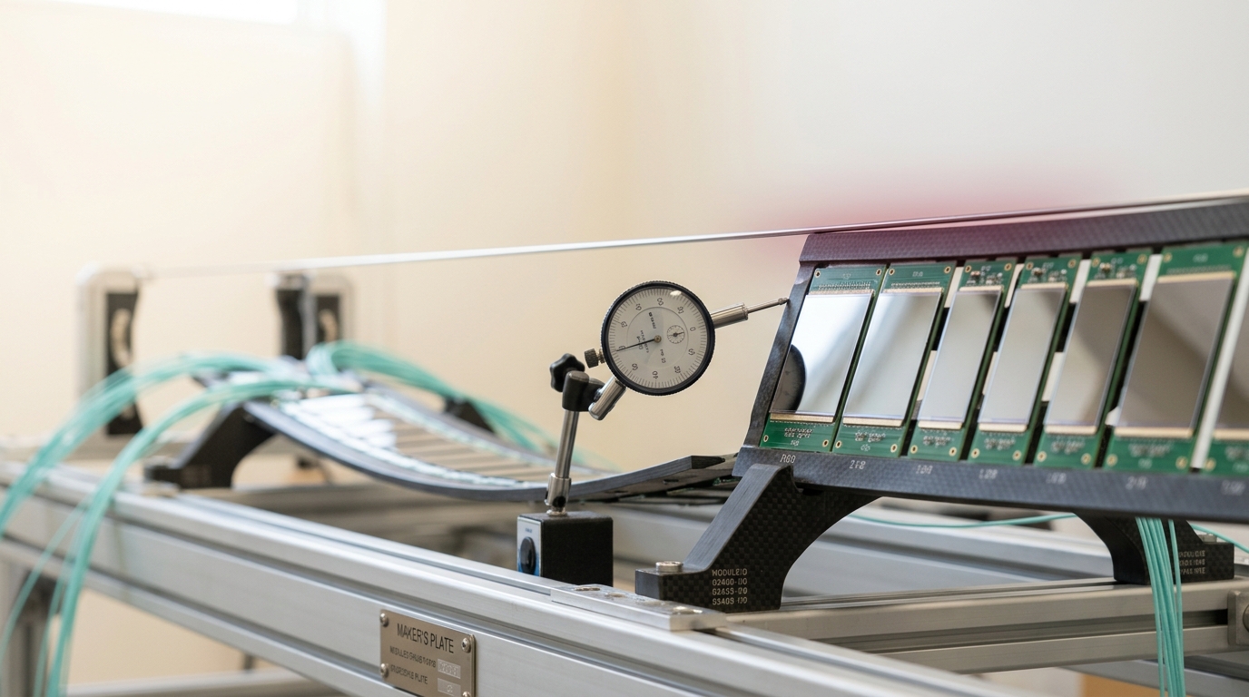
Second, since the sagitta scales with the square of the path length but only linearly with field strength, it is more effective to enlarge the magnetic volume than to raise the field [2]. That single inequality explains why collider detectors are the size of buildings.
Measured performance follows the scaling. In CMS, isolated muon transverse-momentum resolution is about 2.8 per cent at one hundred giga-electronvolts within the central region, with transverse and longitudinal impact-parameter resolutions of roughly ten and thirty micrometres and primary-vertex resolutions of ten to twelve micrometres [7]. Those numbers are not properties of muons. They are properties of a particular silicon geometry inside a particular field, understood to a particular level.
The trigger is an irreversible decision made before understanding
The most consequential stage of the chain happens first, in microseconds, and cannot be revisited.
At the LHC, bunches cross at about forty megahertz. The ATLAS first-level trigger accepts events at up to one hundred kilohertz — the maximum detector readout rate — within a fixed latency of 2.5 microseconds, and the full two-level system records physics collisions at an average of about one kilohertz [5]. The arithmetic is stark: of forty million crossings per second, roughly one thousand are kept. Everything else is not merely unanalysed; it is never read out of the front-end electronics at all. There is no archive of rejected events.

The decision is made on coarse quantities available within the latency budget: energy sums in calorimeter regions, multiplicities of objects above transverse-momentum thresholds, and topological combinations such as invariant masses or angular separations between trigger objects [5]. These are cheap criteria applied to a crude representation of the event. Nothing has been reconstructed; nothing has been identified.
This is a physics-motivated choice, and it is worth being explicit about what it implies. A trigger menu — in ATLAS Run 2, approximately fifteen hundred individual event selections — is a written statement of what the collaboration expects new physics to look like [5]. Signatures outside the menu are not merely difficult to find later. They are absent from the recorded dataset. A process producing only low-momentum, unclustered, prompt hadronic activity is invisible not because the detector cannot see it but because the trigger declined to keep it, on the basis of a hypothesis formed before the data existed.
The field is aware of this and has responded structurally rather than rhetorically. Two responses are visible in the record. The first is partial-event storage: ATLAS operates a trigger-level analysis stream that keeps only physics objects reconstructed online, at an average event size of 6.5 kilobytes against roughly one megabyte for a full physics event, which permits far higher accept rates within the same bandwidth [5]. The second is to abolish the online–offline distinction altogether. LHCb rebuilt its trigger so that offline-quality reconstruction happens in real time, supported by alignment and calibration performed during data taking, which enabled the widespread use of real-time analysis in Run 2 [6]. Both approaches trade retained information for retained events. Neither removes the underlying constraint: a selection rule is applied irreversibly, and the recorded dataset is that rule’s image.
Reconstruction is inference under a model of the detector
What survives the trigger is a list of channel readings. Turning that into objects requires a model of the apparatus, and the model is doing a great deal of work.
Track finding begins with seeds — a few hits compatible with a plausible trajectory — then builds trajectories by gathering compatible hits layer by layer, then fits to extract origin, transverse momentum and direction. The standard implementation is a combinatorial track finder built on Kalman filtering [7]. A Kalman filter is explicitly an inference procedure: it propagates a state estimate and its covariance through a medium whose scattering and energy-loss properties are assumed, and updates that estimate against each measurement. The propagation model — how much material sits between layers, how it scatters — is an input, not an output. Get the material budget wrong and the fitted momenta are wrong in a way no amount of data will reveal.
The same logic governs the step from tracks and clusters to particles. Particle-flow reconstruction identifies a charged hadron by a geometric link between a track and one or more calorimeter clusters together with the absence of a signal in the muon detectors; photons and neutral hadrons are identified as clusters with no linked track [8]. Every one of those statements is a hypothesis test against a detector model. “No track link” means no track was reconstructed, which is not the same as no charged particle having been present. Tracking efficiency in CMS reaches about 94 per cent for pseudorapidities below 0.9 and 85 per cent in the more forward region for particles above 0.9 giga-electronvolts, with the dominant inefficiency arising from nuclear interactions in tracker material [7]. That residual inefficiency does not disappear; it is converted into neutral energy by the reconstruction, because the algorithm has no other category for it.
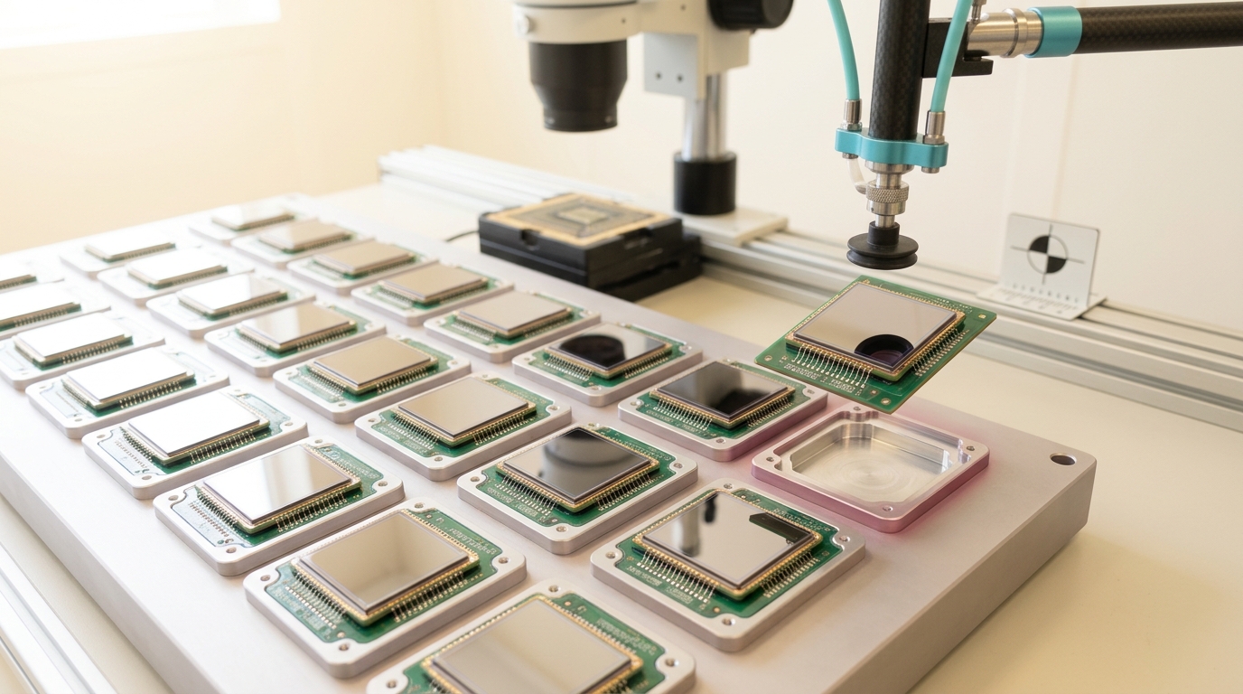
The payoff is real and measurable. Combining the tracker measurement with calorimetry gives far better jet energy resolution than calorimetry alone, where charged-hadron energy is measured with a stochastic term of about 110 per cent divided by the square root of the energy in giga-electronvolts, combined with a nine per cent constant term [8]. But the improvement is bought by trusting the detector model more, not less. Reconstruction does not reduce model dependence; it concentrates it.
Simulation is the bridge, and it carries the corrections
Theory predicts cross-sections and distributions for particles that no detector can register. Detectors register charge, light and time. Simulation is what connects the two, and it is not an accessory to the measurement — it is a load-bearing component of it.
A modern simulation infrastructure chains event generators, a Geant4-based simulation of the response of each detector, digitisation of that response into the same format the real electronics produce, and simulation of the trigger itself, with validation tools that compare simulated output against known physics processes [9]. The output is a synthetic dataset that has passed through the same selection and reconstruction as the real one.
This is where the corrections come from. A published cross-section has roughly the structure
where the numerator is an observed count minus an estimated background and the denominator contains acceptance, efficiency and integrated luminosity. Of the four quantities on the right, only the raw observed count is straightforwardly measured. The background estimate, the acceptance and the efficiency are all obtained from, or heavily constrained by, simulation.
Consider what acceptance means concretely. It is the probability that a process of the assumed kind would have produced an event passing the trigger and reconstruction. That probability is computed by generating the process, pushing it through the simulated apparatus, and counting. It is therefore conditional on the generator being right about the kinematics, on the material model being right, on the trigger emulation matching the deployed trigger, and on the efficiency corrections applied to simulation being valid in the region of interest.
The honest statement is that a cross-section is a statement about nature given a simulation. Collaborations do not pretend otherwise; they measure efficiencies in data wherever a clean control sample exists, derive scale factors between data and simulation, and propagate the residual disagreement as an uncertainty. But the structure remains: the more exotic the signature, the fewer control samples exist, and the more the correction rests on the model rather than on measurement. Searches for the strange are exactly where the simulation is least constrained.
The statistics convert an excess into a claim
Given a spectrum and a background model, the standard machinery is a profile likelihood ratio, with systematic uncertainties represented by nuisance parameters inside the model rather than added afterwards [4, 10]. Asymptotic formulae let the distribution of the test statistic be obtained without extensive simulation, and the Asimov dataset — a representative artificial dataset — supplies median expected sensitivity and the spread around it [10]. The output is a p-value: the probability, under the background-only hypothesis, of a fluctuation at least as extreme as the one observed.
That p-value is conventionally translated into a number of standard deviations. A significance of five corresponds to a p-value of 2.87 in ten million [4]. Two corrections must be applied before the number means anything.
The first is the look-elsewhere effect. A search that scans a mass range does not test one hypothesis; it tests many, and the probability of a fluctuation somewhere in the range is far larger than the probability at any fixed point. Gross and Vitells showed how to quantify the trial factor, which asymptotically grows linearly with the fixed-mass significance [11]. The consequence is that local and global significance can differ dramatically. The ATLAS diphoton search on 2015 data found a local significance of 3.8 to 3.9 standard deviations near 750 giga-electronvolts, but a global significance of only 2.1 standard deviations once the scan was accounted for [16]. The excess did not survive further data. It had, however, already generated a large theoretical literature — a useful reminder that the local number is the one that travels and the global number is the one that matters.
The second correction is judgement, and it is why the threshold is five and not two. Lyons sets out the traditional arguments explicitly: a history of three- and four-sigma effects that vanished with more data; the look-elsewhere effect; a “subconscious Bayes factor” reflecting that an extraordinary claim competes against a very low prior; and the difficulty of estimating systematic uncertainties [12]. The systematics argument is the sharpest. If systematic uncertainties were underestimated by a factor of two, a nominal five-sigma claim is really 2.5 sigma, and the p-value rises by a factor of about twenty thousand [12]. The five-sigma convention is not a statement that physicists demand one-in-three-million certainty. It is a margin held in reserve against the possibility that the error model itself is wrong.
Lyons also argues against applying the threshold uniformly, on the grounds that the look-elsewhere effect, prior plausibility and systematic sensitivity all vary enormously between searches [12]. The PDG review makes a compatible point from the other direction: one’s actual degree of belief depends on the plausibility of the signal hypothesis, on confidence in the model that produced the p-value, and on multiplicity corrections [4]. There is no consensus that a single threshold is correct; there is a working convention that is defended as conservative rather than as principled. Characterising that disagreement accurately is more useful than resolving it.
Systematic uncertainty is usually the term that decides
For a mature measurement, the statistical error is the easy part. It shrinks predictably with more data and its distribution is known. The systematic term does neither.

The scale of correction work involved is easy to underestimate. In the Fermilab measurement of the positive muon anomalous magnetic moment, the ratio of measured frequencies must be corrected for beam dynamics, magnetic transients, calibration and several other effects, and those corrections shift the result by 622 parts per billion in total, against a final total uncertainty on the anomaly of 215 parts per billion [17]. The corrections are nearly three times the size of the quoted error. Everything depends on their being right.
That measurement is also an honest counterexample to a lazy generalisation. Its dominant uncertainty on the precession frequency is statistical — 201 parts per billion against 25 parts per billion of systematic — which is precisely why the experiment continued taking data [17]. “Systematics always dominate” is false as stated. The accurate version is that systematics dominate once statistics have been reduced far enough, and that this crossover is where most long-running measurements spend their lives.
At the LHC the crossover often arrives immediately. Both 2012 Higgs observation papers quote mass uncertainties in which the systematic term already equals or exceeds the statistical one: ATLAS reported 126.0 with 0.4 statistical and 0.4 systematic, CMS 125.3 with 0.4 statistical and 0.5 systematic, in giga-electronvolts [14, 15]. The same structure appears in calorimetry, where the constant term — construction tolerance, electronics stability, calibration — sets the floor at high energy [2].
Where do those systematic terms come from? Luminosity calibration, energy and momentum scale calibration, efficiency scale factors between data and simulation, background modelling, generator choice, parton distribution functions, and detector material budget. Every one of them is an inference-chain quantity. None of them is a property of the collision. The modern statistical treatment absorbs them as nuisance parameters constrained by auxiliary measurements [4], which is methodologically clean but does not remove the underlying problem: a systematic uncertainty is a statement about how wrong the model might be, and it is estimated using the model.
Blinding is a procedural defence, not a statistical one
The final link in the chain is the analyst, and the field’s response to that link is procedural rather than mathematical.
The motivation is documented rather than theoretical. Klein and Roodman collect the evidence: Dunnington in 1932 deliberately kept himself ignorant of the angle in his electron charge-to-mass measurement by asking his machinist to build the apparatus close to, but not exactly at, the required 340 degrees, so that he could not compute his own answer prematurely; the series of speed-of-light measurements from 1930 to 1940 sits about 17 kilometres per second from the modern value; and across a set of historical measurements of the neutron lifetime, the neutral kaon lifetime and related quantities, the data cluster nearer the previously published averages than the eventual values, with a chi-squared of 131.2 for 83 degrees of freedom about the prior averages against 249.7 for about 82 degrees of freedom about the final ones [13]. The authors are careful, and so should any reader be: this is circumstantial, and alternative explanations such as shared methodological errors are available. But the mechanism is plausible and cheap to defend against.
The defence is to make the answer unavailable while the analysis is being fixed. Klein and Roodman classify the techniques: hiding the signal region entirely, hiding the answer behind an offset, adding or removing events, and prescaling the data [13]. The practice in nuclear and particle physics dates from around 1990, with a Brookhaven rare-decay search that had an obvious incentive — a discovery could easily be lost if final cuts were tuned to remove events sitting awkwardly near the edge of the signal box [13].
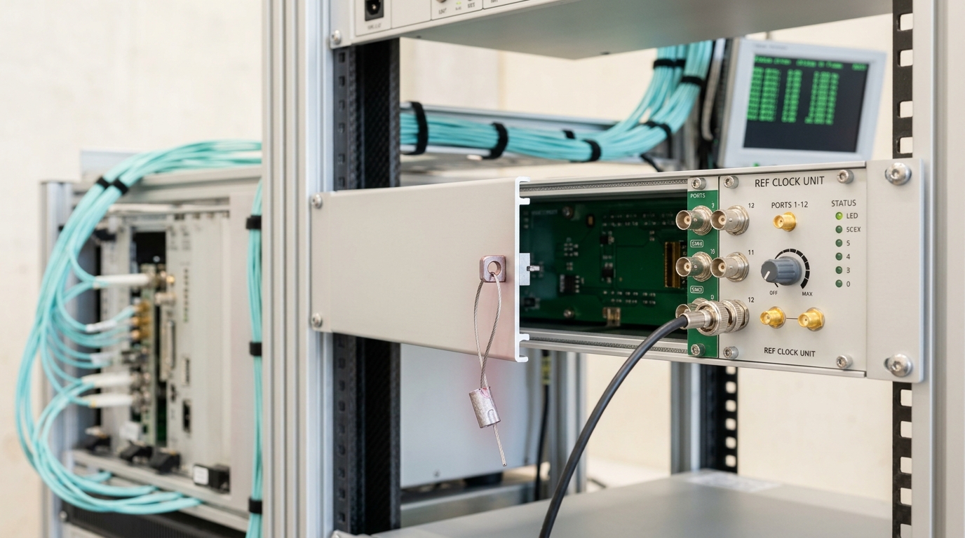
The muon g-2 measurement shows what a serious implementation looks like now. The data are blinded by hiding the true value of the calorimeter digitisation clock frequency, so that the extracted precession frequency is offset by an amount nobody in the collaboration knows; on top of that, seven independent analysis groups each add their own additional blind offset, so that groups cannot converge on one another either; the consistency of the groups’ results and of their independently estimated systematic uncertainties is only assessed after unblinding [17]. Blinding here is not a gesture. It is a hardware configuration and an organisational structure.
What blinding buys is specific and limited. It prevents cuts, corrections and uncertainty estimates from being tuned — consciously or not — toward an expected answer. It does not detect a wrong detector model, a bad generator or an unmodelled background. It defends one link in the chain, and it is the only link for which the failure mode is psychological rather than physical.
Where the uncertainty actually lives
Read back, the chain runs: liberated charge and light, digitised within a fixed latency; a coarse selection rule that discards all but roughly one crossing in forty thousand and cannot be undone; a reconstruction that imposes a model of material, field and geometry on the survivors; a simulation that supplies the acceptance and efficiency without which the count cannot be normalised; a likelihood that turns the corrected count into a p-value; a multiplicity correction and a conservative threshold; a systematic term assembled from calibrations and model comparisons; and a procedural firewall between the analyst and the answer.
The collision itself is the shortest and least contested part of that sequence. It happened, and it is gone. Every subsequent step is a place where a defensible choice was made, and where a different defensible choice would have produced a different number.
This suggests a practical reading discipline for anyone assessing a claim from this field. Ask what the trigger required, because that bounds what could have been found at all. Ask which quantities came from simulation rather than from data, and what control samples constrained them. Ask whether the quoted significance is local or global. Ask whether the systematic uncertainty is dominated by a term whose estimation procedure is itself model-dependent. Ask whether the analysis was blinded, and to what.
None of this is scepticism about the results. The 2012 Higgs observation was reported at 5.9 standard deviations by ATLAS and 5.0 by CMS, in independent apparatus with independent reconstruction chains and independent simulation, and it has held [14, 15]. That agreement is meaningful precisely because the two chains were different; the collision was common, but almost nothing else was. The lesson is not that the inference chain is untrustworthy. It is that the chain, not the collision, is the object about which trust has to be established — and the field’s methodological apparatus, from trigger menus published in full through blind analysis protocols, is best understood as an accumulated set of defences at each link.
Nobody observes a particle. What gets published is a number, a bracket, and a long argument about the machine that produced them.