How Scientific Instruments and Metrology Actually Work

A number is the end of a chain, not the start of one

A displayed reading — 20.0037 grams, 293.152 kelvin, 1.2 angstrom — looks self-contained. It is not. Every scientific instrument in routine use reports a number that is only meaningful because it can be related, through a documented sequence of comparisons, to a standard that the whole world has agreed to treat as fixed. That sequence is called a metrological traceability chain, and it is the subject this new series on scientific instruments and metrology opens with, because almost nothing else in the series makes sense without it. A telescope’s photometric calibration, a mass spectrometer’s isotope ratio, a clinical assay’s reference range, a gravitational-wave detector’s strain readout — all of them terminate, eventually, in the same handful of definitions and the same discipline of comparison.

This article builds that chain from scratch, in three stages that mirror how an actual measurement is made trustworthy: first, how a reading is linked back to an SI-defined unit through calibration; second, how the uncertainty of that link is computed rather than guessed, using the internationally adopted GUM framework; and third, how two instruments that individually claim excellent performance are checked against each other, because a single instrument’s internal consistency is not the same thing as its correctness. A worked example from electron microscopy — an instrument class built almost entirely out of correcting for its own physical limitations — runs through all three stages as a concrete case.

Throughout, four registers are kept separate on purpose: fact (a defined constant, a published equation, a documented result), vendor or institutional claim (a stated specification or capability), analysis (an inference this article draws from the facts), and scenario/prediction (a forward-looking claim, always given a horizon, assumptions, and a way it could turn out wrong). Where they mix in the source literature, they are unmixed here.

What “traceable” actually means

The International System of Units defines seven base units — the metre, kilogram, second, ampere, kelvin, mole and candela — each now fixed by declaring an exact numerical value for a fundamental constant of nature, such as the Planck constant for the kilogram or the ground-state hyperfine transition frequency of caesium-133 for the second ^[1]. That definitional layer is fixed at the top of the pyramid and almost never touched directly by a working laboratory.

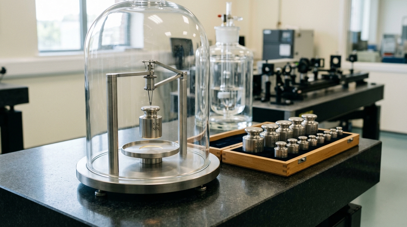
Below it sits a chain of physical realizations. A national metrology institute — NIST in the United States, PTB in Germany, NPL in the United Kingdom, and dozens of counterparts worldwide — maintains primary standards that realize a unit as closely as current technology allows: a Kibble balance realizing the kilogram from the fixed Planck constant, a caesium fountain clock realizing the second. These institutes calibrate secondary reference standards, which calibrate working standards at accredited calibration laboratories, which in turn calibrate the instrument sitting on a bench in an ordinary lab. NIST states the definition precisely: metrological traceability is “the property of a measurement result whereby the result can be related to a reference through a documented unbroken chain of calibrations, each contributing to the measurement uncertainty” ^[4]. Three words in that sentence do all the work — documented, unbroken, and each contributing. A calibration certificate with a gap in its date sequence, an uncalibrated intermediate device, or an uncertainty budget that silently drops a link is not a traceability chain; it is a plausible-looking number.

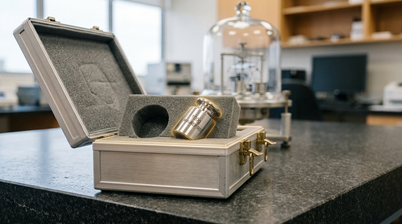
This is why the hero image for this article is a mass comparator moving a reference weight, not a certificate on a wall. Traceability is enforced by a physical act repeated on a schedule: a working reference is periodically carried, in a case, to a laboratory one step closer to the primary standard, compared there under controlled conditions, and returned with an updated correction value and an updated uncertainty. NIST’s own guidance is explicit that traceability is a property of the result, not of the laboratory or the instrument — “a laboratory is not traceable,” in the institute’s own phrasing ^[4]. An instrument does not become trustworthy by being expensive or reputable; it becomes trustworthy because a specific number it produced can be walked back, calibration by calibration, to a definition.

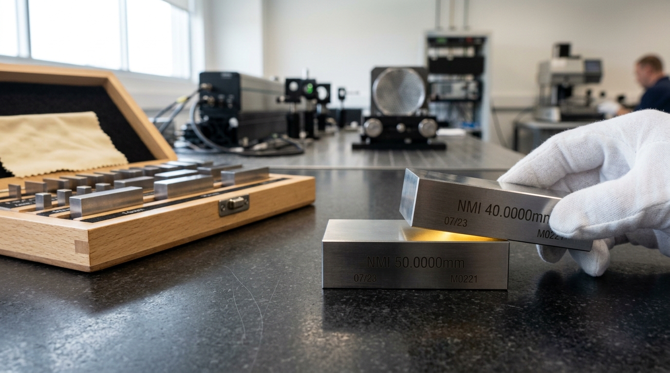
Gauge blocks make the physical discipline behind this concrete. A gauge block is a small rectangular steel or ceramic block lapped so flat and so parallel on its two working faces that another block can be “wrung” onto it — slid into intimate optical contact until the two behave as one longer block, held together by nothing but the near-total absence of any gap between their surfaces. The certified length of a gauge block is traceable to the metre through laser interferometry, and its practical usefulness as a working length standard for machine shops and calibration labs depends entirely on that flatness and parallelism holding to a fraction of the wavelength of light being used to measure it.

A fixed point of a physical constant does similar work for temperature. A triple-point-of-water cell — a sealed glass vessel containing pure water at the unique combination of pressure and temperature where solid, liquid and vapor phases coexist — defines 273.16 K exactly by construction, provided the ice mantle inside is grown and maintained correctly. Reference thermometers are calibrated against such fixed points rather than against an arbitrary previous thermometer, which is precisely how the chain avoids compounding drift indefinitely as it is handed down from primary standard to bench instrument.

Calibration produces a correction, not a device you trust more

Calibration is often misdescribed as an act of making an instrument more accurate. It does not change the instrument’s underlying physics at all. Calibration is the act of comparing an instrument’s output to a known reference under stated conditions and recording the relationship between the two — typically as a correction value or a calibration curve, always accompanied by an uncertainty. An instrument is not “calibrated to be accurate”; it is calibrated so that its systematic bias, at the time of calibration, under the conditions of calibration, is known and can be corrected for. Between calibrations, that known bias can drift, which is why calibration intervals exist and why a calibration certificate carries a date and, implicitly, an expiry of confidence.

This is also where the difference between accuracy and precision stops being a classroom slogan and becomes an operational distinction. A balance that reports the same mass to six decimal places on every repeat weighing is precise; whether it is accurate depends entirely on whether its calibration correction has been applied and is still valid. NIST’s foundational technical note on measurement uncertainty was written specifically because engineers and scientists were treating “precise” and “accurate” as interchangeable when only a documented calibration and uncertainty statement can distinguish them ^[3].

Turning a list of error sources into one number: the GUM framework

Once a calibration correction exists, the remaining question is how confident to be in it — and in every measurement made using the now-corrected instrument. The internationally adopted answer is the Guide to the Expression of Uncertainty in Measurement, universally known by its acronym GUM, published by the Joint Committee for Guides in Metrology and endorsed by the BIPM among other international bodies ^[2]. Before the GUM, laboratories used inconsistent, often incompatible conventions for combining error sources — some added them linearly, some quoted only the largest one, some simply omitted sources they could not easily quantify. The GUM’s contribution was not a new physical insight; it was a common accounting method, so that an uncertainty quoted by one laboratory means the same thing as an uncertainty quoted by another.

The GUM’s central move is to treat every measured or estimated quantity a result depends on as a random variable with its own estimated standard uncertainty, and then to propagate those uncertainties through the mathematical relationship that produces the final result. If a measurement result $y$ is a function of $N$ input quantities, $y = f(x_1, x_2, \ldots, x_N)$, the combined standard uncertainty is obtained from a first-order Taylor expansion of that function:

The first sum is the familiar root-sum-of-squares combination of independent contributions, each weighted by how sensitive the final result is to that input (the partial derivative, or “sensitivity coefficient”). The second sum is easy to forget and often the source of a badly wrong uncertainty budget: it accounts for covariance between input quantities that are not independent — for example, two lengths measured with the same miscalibrated ruler share a correlated error, and ignoring that correlation can make a combined uncertainty either too small or too large depending on the sign of the correlation ^[2].

The GUM also formalizes a distinction that predates it but that it made rigorous: Type A uncertainty evaluation is a statistical analysis of a series of repeated observations — a standard deviation of repeated readings, essentially. Type B evaluation covers everything else contributing to uncertainty that is not estimated from repeated measurement: a manufacturer’s stated tolerance on a calibrated weight, a known but uncorrected environmental sensitivity, a published uncertainty inherited from the reference standard’s own calibration certificate. Both types are combined in the same equation above; the GUM’s insight was that the distinction is about how an uncertainty is evaluated, not about which contributions are more legitimate to count. A Type B component from a calibration certificate is exactly as real as a Type A component computed from twenty repeat weighings, and a budget that includes only the latter because it is easier to compute is an incomplete budget, not a conservative one.

Fact: the GUM framework, and the $k_{\mathrm B}$-free equation above, applies to any measurement expressible as a function of quantifiable inputs; it makes no claim about which physical effects matter for a given instrument — that judgment is the analyst’s, and getting it wrong (omitting a real contributor, or including a negligible one to pad the budget) is the most common failure mode in practice, one NIST’s own technical note spends most of its length trying to prevent ^[3].

The electron microscope: buying resolution back from physics

An electron microscope is a useful worked example precisely because almost the entire modern instrument exists to correct for a limitation baked into its own optics. The achievable resolution of any imaging system with a circular aperture is bounded, in the simplest diffraction-limited approximation, by a form of the Rayleigh criterion:

where $\lambda$ is the wavelength of the illuminating radiation, and $n\sin\alpha$ is the numerical aperture of the imaging system. For visible light this caps optical microscopy at roughly 200 nanometres — far too coarse to resolve individual atoms, whose spacing in a solid is typically a few tenths of a nanometre. Electron microscopy exploits the far shorter de Broglie wavelength of accelerated electrons — picometre scale at typical accelerating voltages — to push the diffraction limit itself down by more than three orders of magnitude.

That would already be enough to reach atomic resolution on the diffraction limit alone, but a second, older problem intervenes: unlike a glass lens, an electromagnetic lens used to focus an electron beam suffers from spherical and chromatic aberration that is far harder to correct, and for decades this aberration — not the diffraction limit — was the practical ceiling on resolution. Fact: the introduction of hardware aberration correctors, multipole electromagnetic elements inserted into the microscope column that actively cancel the dominant aberration terms, was what allowed transmission electron microscopes to approach and then exceed diffraction-limited resolution predictions from the pre-corrector era, with aberration-corrected instruments demonstrating single-atom imaging and sub-ångström resolution in the 2000s ^[8].

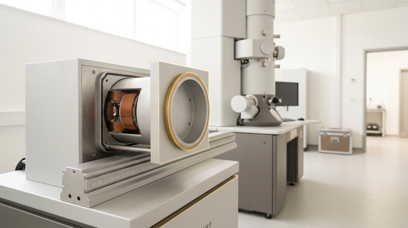
Analysis: the more recent advance beyond hardware aberration correction is computational. Electron ptychography reconstructs a specimen’s structure from a full four-dimensional diffraction dataset — recording the diffraction pattern at every scan position rather than a single intensity value — and uses an iterative phase-retrieval algorithm to recover information that a physical lens, however well corrected, discards. Using this approach on a monolayer material, one study demonstrated resolution below 0.5 ångström, deeper than the resolution achievable by the same instrument’s physical optics alone, effectively trading detector dynamic range and computation for lens quality ^[7]. This is worth stating carefully as a scope-limited result rather than a general claim about all electron microscopy: it was demonstrated on a thin, well-ordered two-dimensional specimen under specific beam and detector conditions, and the improvement over conventional imaging depends on exactly that combination of very thin sample and very high dynamic range detection. It does not follow that every electron-microscopy measurement on every specimen now reaches sub-ångström resolution.

A microscope’s stated resolution is, in metrological terms, itself the output of a calibration and uncertainty exercise. Manufacturers publish a specification (a vendor claim) for a given accelerating voltage and corrector configuration; an operating laboratory verifies it against a calibration specimen with a known lattice spacing, under its own vibration, thermal and magnetic-field conditions, and reports an achieved resolution with its own uncertainty rather than simply repeating the datasheet figure. The two numbers can differ substantially, and a laboratory that reports the vendor specification as its own achieved performance without independent verification has skipped exactly the traceability step this article opened with.

Spectroscopy and the comb that connects frequencies to counting

Optical spectroscopy — inferring atomic and molecular structure from the frequencies of light absorbed or emitted — depends on being able to state a measured frequency in SI units with a known uncertainty, and optical frequencies (hundreds of terahertz) are far too fast for electronic counters to measure directly. The practical solution is the optical frequency comb: a laser source, usually a mode-locked femtosecond laser, whose output spectrum consists of a series of extremely sharp, evenly spaced frequency lines — the “teeth” of the comb — with a spacing and an offset that can themselves be measured and controlled with a radio-frequency reference. An unknown optical frequency is compared against the nearest comb tooth, and the resulting radio-frequency beat note is something an ordinary electronic counter can measure directly, giving the optical frequency in terms of a countable, traceable radio-frequency standard.

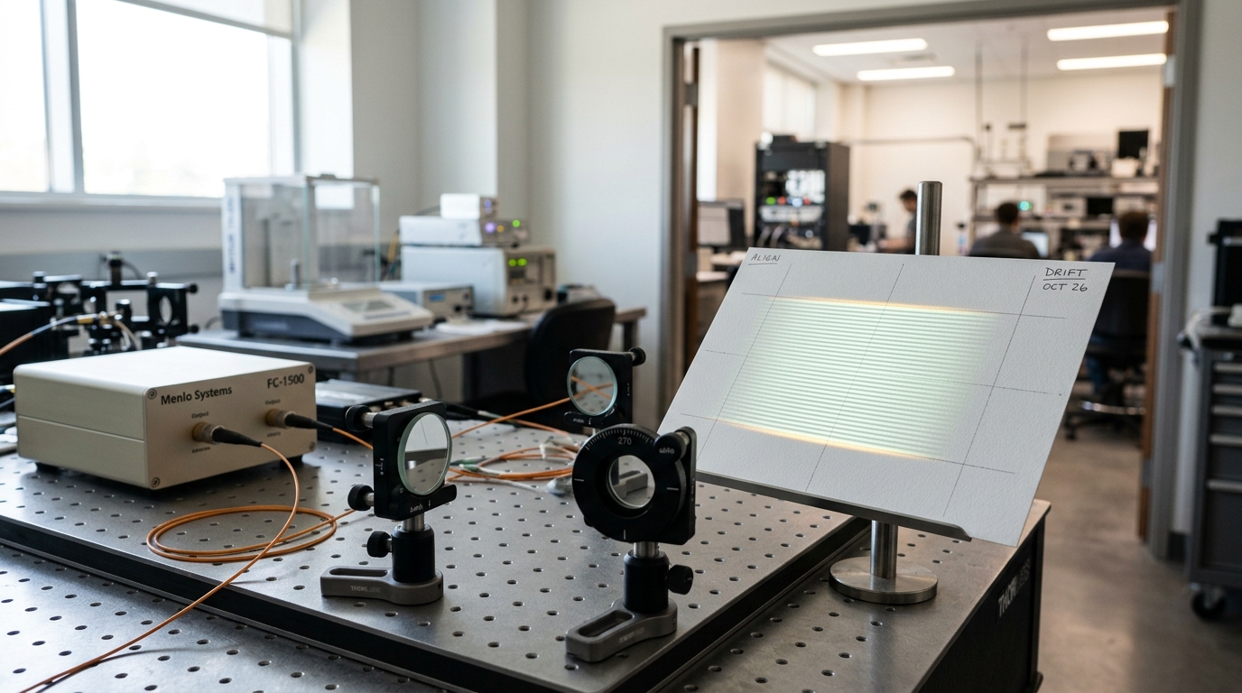
This is the same traceability principle as the mass comparator and the gauge block, applied to frequency rather than length or mass: an inaccessible quantity (an optical frequency, an unknown mass) is compared directly against a reference whose own value is already tied to the SI definition, rather than measured in some absolute sense from first principles each time. The 2019 redefinition of the SI in terms of exactly fixed fundamental constants — including the exact numerical value now assigned to fix the second via the caesium hyperfine transition, and constants such as the molar gas constant now derived rather than separately measured ^[6] — did not change how any of these comparison techniques work day to day; it changed what sits at the top of the chain they all eventually reach ^[1].

Reproducibility is checked between labs, not assumed within one

An instrument’s internal consistency — the same reading recurring on repeat measurement — says nothing about whether that reading is correct, because a systematic error recurs just as reliably as a correct measurement does. The standard check against this is the interlaboratory comparison: two or more laboratories measure the same artefact, or nominally identical artefacts, and compare results with their stated uncertainties. Internationally, the CIPM Mutual Recognition Arrangement formalizes this at the highest level: national metrology institutes participate in “key comparisons,” coordinated by the BIPM and its consultative committees, in which the same reference artefact is circulated among institutes and each institute’s result is checked against the others for consistency with its own claimed uncertainty ^[5]. The outcome of a key comparison is not a ranking of “best” laboratory; it is a statement of the degree of equivalence between each institute’s realization of a unit, which is exactly what allows a calibration certificate issued in one country to be trusted in another.

Analysis: the practical value of this system is that it catches a specific failure mode no single laboratory can catch on its own — a systematic bias shared by every instrument of one laboratory’s design or lineage, invisible from repeat measurements within that laboratory because the bias is the same every time. A comparison result in which one institute’s measured value falls outside the combined uncertainty interval of the group is a signal that either that institute’s stated uncertainty was too small, or an unrecognized systematic effect is present, or both — and either finding is more useful to the field than a comparison that simply confirms everyone agrees, because most comparisons that matter are the ones that surface a discrepancy.

This is the general lesson the rest of this series will return to for each specific instrument class: precision within one measurement chain is necessary but not sufficient, and the comparisons that expose a hidden systematic bias are usually inconvenient, occasionally embarrassing to a specific laboratory, and exactly the mechanism by which measurement science is kept honest rather than merely internally self-consistent.

Scenario: what changes and what does not, going forward

Scenario, five-to-ten-year horizon: as more national metrology institutes shift primary realizations of the kilogram, ampere and mole to quantum-electrical and Kibble-balance methods rather than physical artefacts, and as optical atomic clocks mature toward a possible future redefinition of the second, the number of physical steps between a bench instrument and the top of its traceability chain is likely to shorten for some quantities, because quantum-based realizations can sometimes be implemented directly at a national institute or even a well-equipped university lab rather than requiring an artefact literally carried from a central vault. This is an extrapolation, not a settled fact: it assumes continued investment in quantum-based primary standards, continued agreement among national institutes on any further redefinition, and no major disruption to the comparison infrastructure that currently validates equivalence between institutes. An observable indicator that this scenario is unfolding would be a measurable decline in the average number of calibration links in typical accredited traceability certificates over that period; the scenario would be disconfirmed if key comparisons continued to show physical artefact transfer as the dominant calibration route for these quantities a decade from now.

What will not change, on the same horizon, is the underlying discipline: a documented, unbroken chain of comparisons, an uncertainty computed rather than asserted, and periodic comparison against an independent chain. Those three requirements are not specific to any one technology or unit definition, which is exactly why they are the foundation this series on scientific instruments and metrology starts from before turning, in later pieces, to what specific instrument classes do with that foundation.