From Origins to Frontier: A History of Systems and Computational Neuroscience

Systems and computational neuroscience does not have a founding theory the way thermodynamics has its laws or genetics has Mendel’s ratios. It has a founding instrument problem: the brain is made of components too small, too fast, and too numerous to observe directly, and almost every major advance in the field’s seventy-year history is really the story of a new way to make one piece of that problem observable. This is a history of those instruments — what each one actually measured, what it could not, and how the interpretive claims built on top of the data have grown more ambitious than the data themselves.

Fact: one axon, one equation (1952)

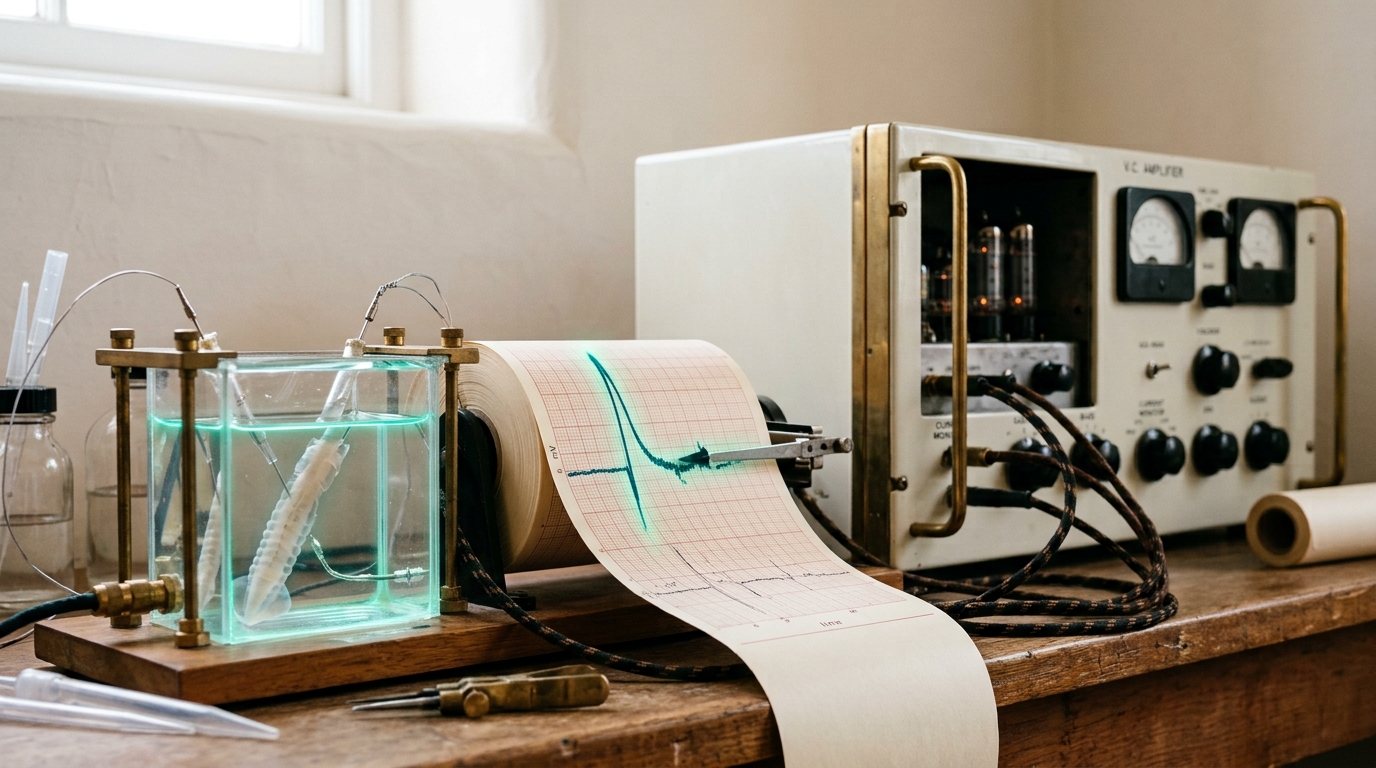
In 1952, Alan Hodgkin and Andrew Huxley published a set of papers in The Journal of Physiology built on voltage-clamp recordings from the giant axon of a squid, a preparation large enough — nearly a millimeter in diameter — that electrodes of the day could be threaded down its length ^[1]. By holding the membrane potential fixed and measuring the current required to hold it there, they separated the total membrane current into sodium and potassium components and fit each to a set of coupled nonlinear ordinary differential equations describing voltage-dependent conductance. The result, now called the Hodgkin-Huxley model, reproduced the shape, threshold, and propagation velocity of the action potential from first principles rather than by curve-fitting an already-observed waveform.

The model’s core equation describes membrane current as the sum of capacitive, sodium, potassium, and leak components:

where $m$, $h$, and $n$ are voltage- and time-dependent gating variables each obeying their own first-order kinetics. This is worth stating in full because it is the paradigm the rest of the field either extends or reacts against: a biophysical mechanism, expressed as a dynamical system, fit to directly measured current, with no free parameter standing in for an unmeasured process. It is why the model is still taught unmodified, and why its two authors and John Eccles shared the 1963 Nobel Prize in Physiology or Medicine. It is also, strictly, a model of one excitable membrane, not of a circuit, a computation, or a behavior — the questions that would define the next seventy years were exactly about what happens when this unit is multiplied by billions and wired into structure.

Fact: mapping structure onto function, one column at a time (1959-1962)

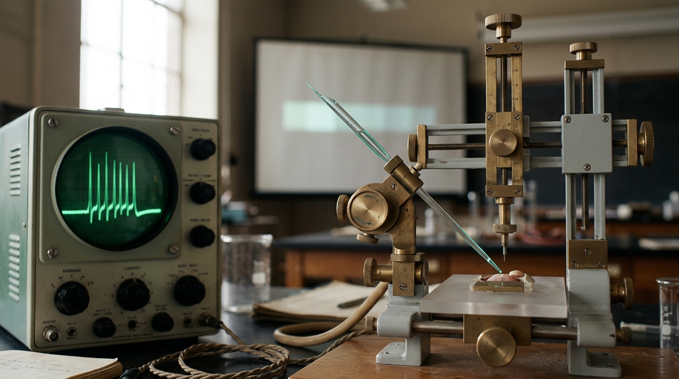
The next foundational instrument was not new hardware so much as a new use of an existing one — extracellular recording with a fine glass or metal microelectrode, pushed into the cortex of an anesthetized cat while a bar or edge of light was swept across a screen in front of its eyes. David Hubel and Torsten Wiesel used this method through the late 1950s and published its full picture in 1962: neurons in primary visual cortex responded not to spots of light, as retinal ganglion cells do, but to oriented edges at specific locations, and neurons with similar orientation preference were arranged in vertical columns through the cortical layers ^[2]. This was the first demonstration that a piece of neocortex has a discoverable functional architecture — that its wiring is not a uniform mesh but a structured map that an experimenter, electrode in hand, could actually chart cell by cell. Hubel and Wiesel shared the 1981 Nobel Prize (with Roger Sperry) for this and the subsequent work on cortical development it enabled.

The method generalized far beyond vision. Two and a half decades later, Apostolos Georgopoulos, Andrew Schwartz, and Ronald Kettner recorded from populations of motor cortex neurons in monkeys reaching in different directions and showed that no single neuron’s firing rate reliably specified movement direction, but a weighted vector sum across the population — each cell’s activity weighted by its own preferred direction — pointed accurately at the direction actually moved ^[4]. This “population vector” result reframed the field’s basic unit of analysis: from what one neuron signals to what a population jointly represents, a shift that underlies every modern neural-decoding and brain-computer-interface algorithm. It is worth being precise about what the result does and does not show: it demonstrates that direction is linearly decodable from a population under this task and this decoding rule; it does not by itself establish that the motor cortex computes movement this way, only that this particular readout recovers the behavioral variable with high fidelity. Later work has debated how literally to interpret the vector-sum construction as the brain’s own mechanism versus as an effective description — a distinction the original paper’s authors were careful about and that is frequently flattened in later summary.

Fact: a complete wiring diagram, one worm at a time (1986)

While cortical physiology was mapping function onto electrode position, a separate program was mapping structure exhaustively rather than sampling it. John White, Eileen Southgate, J. Nichol Thomson, and Sydney Brenner spent over a decade reconstructing the nervous system of the nematode Caenorhabditis elegans from thousands of serial-section electron micrographs, tracing every neurite by hand across successive thin sections and cataloguing every synapse ^[3]. The 1986 paper reported the complete wiring diagram of all 302 neurons of the hermaphrodite worm — the first, and for decades the only, full connectome of any animal’s nervous system. This is the direct methodological ancestor of every connectomics project that followed: the same principle — physically section tissue, image every section, trace every process across sections, reconstruct the graph — scaled from one worm’s 302 neurons to a fly’s 139,255 four decades later, at a cost in labor and image data that grew by many orders of magnitude for each step up in organism complexity.

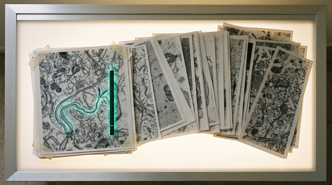
It is a fact, not an inference, that having this wiring diagram did not by itself explain the worm’s behavior. Structural connectivity constrains but does not determine dynamics — synaptic weight, neuromodulation, and extrasynaptic signaling are not fixed by the anatomical graph — and C. elegans behavioral neuroscience has continued for decades past 1986 precisely because the map was a necessary but not sufficient foundation. This is the first clear instance of a pattern that recurs at every later scale increase in connectomics: a complete map answers “what is wired to what” and leaves “what does the wiring do” as a separate, harder question.

Fact: a new organ becomes visible without surgery (1990)

Every method described so far required opening the skull. In 1990, Seiji Ogawa, Tso-Ming Lee, Alan Kay, and David Tank, working at AT&T Bell Laboratories, showed that deoxygenated hemoglobin’s magnetic properties produced a measurable contrast in gradient-echo magnetic resonance images of the rodent brain, and that this contrast tracked physiological manipulations of blood oxygenation such as altered inspired oxygen ^[5]. This blood-oxygen-level-dependent, or BOLD, contrast is the physical basis of functional MRI as practiced today: it does not measure neural activity directly but measures a hemodynamic consequence of the local metabolic demand that follows it, with a lag of several seconds and a spatial resolution set by the vasculature rather than by individual neurons. Within a few years BOLD imaging was extended to humans performing cognitive tasks, and by the 2000s it had become the dominant noninvasive method for localizing task-related activity across the whole human brain.

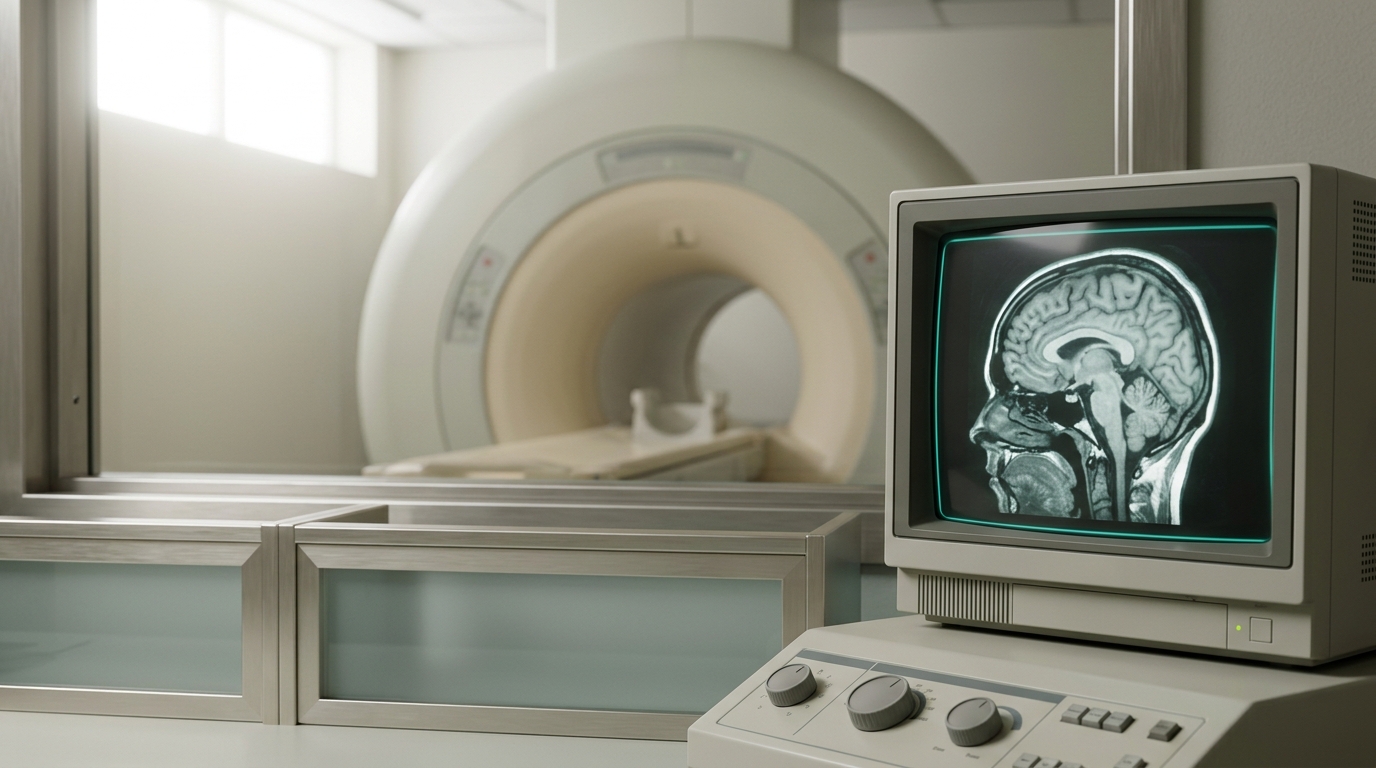
The technique’s popularization brought with it a specific and well-documented inferential risk, worth stating as an explicit analytic caution rather than a fact about the method itself: a BOLD signal increase in a region during a task is evidence that blood flow to that region changed, which is evidence consistent with increased local neural activity, but the chain from voxel to cognitive process passes through several non-trivial steps — hemodynamic coupling, statistical thresholding across tens of thousands of voxels, and the researcher’s choice of contrast condition — each of which can distort the final localization claim if handled carelessly. The field’s own methodological literature, not outside critics, produced the strongest corrections to overreading single-study fMRI maps as clean readouts of function. The 2013 launch of the Human Connectome Project, led by David Van Essen and Kamil Ugurbil among others, was itself partly a response to this: a large, standardized, multimodal acquisition (structural MRI, diffusion imaging, resting-state and task fMRI, MEG) across hundreds of healthy adults, designed so that individual differences in structural and functional connectivity could be related to behavior with enough statistical power to survive the multiple-comparisons problem that had undermined smaller single-site studies ^[8].

Fact: turning light into a switch for one cell type (2005)

Electrode recording and lesion studies could show that activity in a region correlated with, or was necessary for, a behavior, but neither method could turn one genetically defined cell type on or off with millisecond precision inside an intact, behaving animal. In 2005, Edward Boyden, Feng Zhang, Ernst Bamberg, Georg Nagel, and Karl Deisseroth showed that channelrhodopsin-2, a light-gated ion channel from the green alga Chlamydomonas reinhardtii, could be expressed in mammalian neurons via lentiviral delivery and used to drive reliable, millisecond-timescale spiking with pulses of blue light ^[6]. Combined with cell-type-specific genetic promoters, this gave experimenters a causal lever that recording alone cannot provide: not “this region is active during the behavior” but “activating this specific population is sufficient to produce, or its silencing is sufficient to interrupt, this specific behavior.” Optogenetics, together with its chemogenetic cousins (DREADDs and related engineered receptors), became the dominant causal-manipulation toolkit in rodent systems neuroscience within a decade of the original paper, extended since to non-human primates.

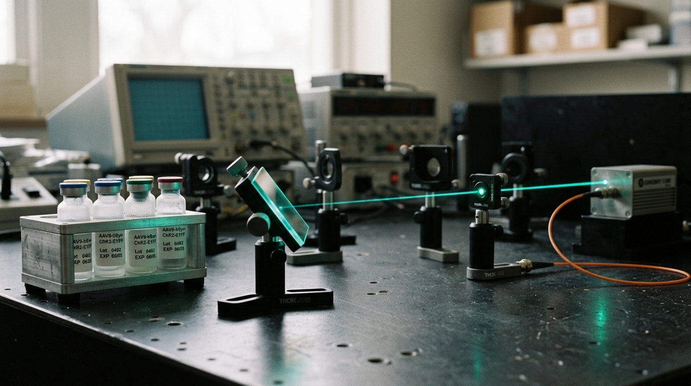
It is important, per the field’s own methodological discussions, to keep “sufficient to produce” and “necessary and naturally used to produce” separate claims. Optogenetic stimulation typically drives synchronous, non-physiological firing patterns in the targeted population; showing that artificially synchronized activity in a cell type can trigger a behavior is not the same claim as showing that the endogenous, naturally patterned activity in that same population is what normally causes the behavior in an intact animal. Most careful papers in the optogenetics literature are explicit about this distinction; it is the summarized, secondhand version of results that tends to collapse “sufficient under artificial stimulation” into “the natural cause.”

Fact: mapping wiring at scale, with function attached (2011-2024)

By the late 2000s, serial-section electron microscopy had been automated far beyond White and colleagues’ hand-tracing: robotic ultramicrotomes could cut thousands of ultrathin sections and mount them for automated imaging, and computer-vision alignment and segmentation software could trace neurites across the resulting image stacks with far less manual labor per neuron. Davi Bock, Wei-Chung Allen Lee, and colleagues combined this with a technique new to the field: recording the functional response properties of a small group of neurons in mouse visual cortex with two-photon calcium imaging first, then relocating and reconstructing the very same neurons’ synaptic wiring with serial-section electron microscopy, directly linking measured function to measured structure in the same cells for the first time at synaptic resolution ^[7].

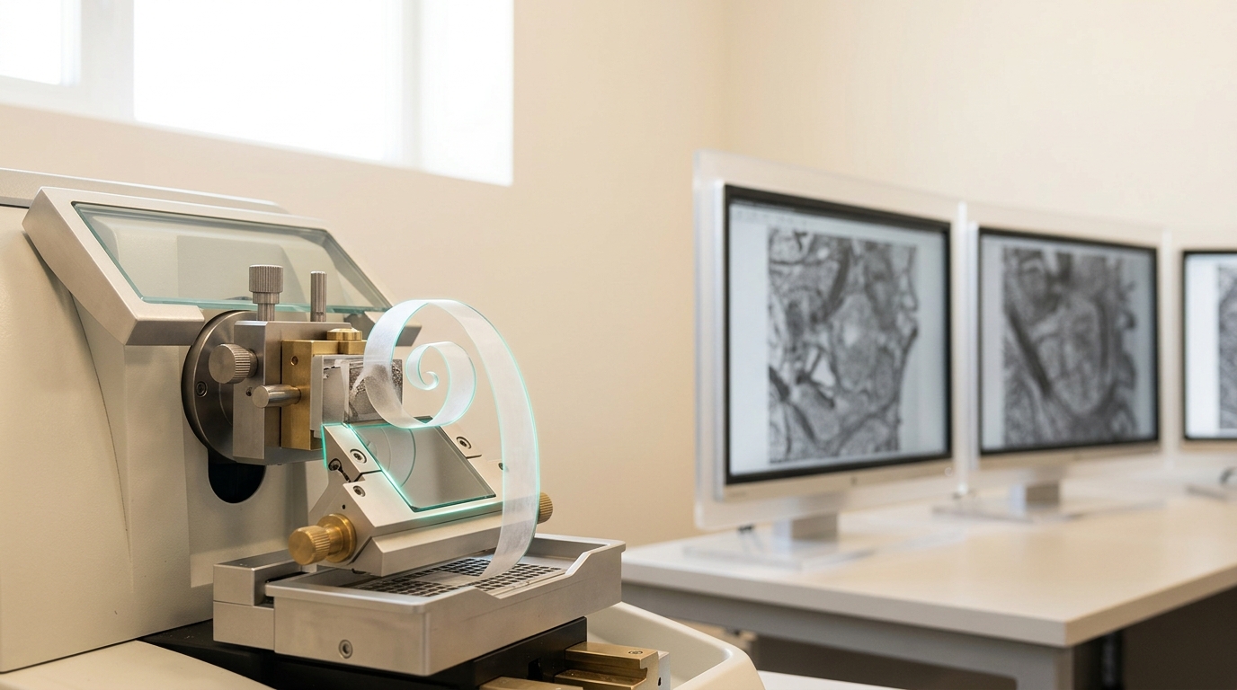
This structure-plus-function approach scaled through the 2010s into large consortium efforts (the Allen Institute’s and international collaborators’ cortical column reconstructions, and separately the MICrONS program) and, in October 2024, into the first connectome of an entire adult brain more complex than C. elegans’s: Sebastian Dorkenwald, Arie Matsliah, and the international FlyWire Consortium published a complete wiring diagram of the adult Drosophila melanogaster brain — 139,255 neurons and roughly fifty million chemical synapses, annotated for cell type, predicted neurotransmitter, and developmental lineage ^[9]. As with the 1986 worm connectome, this is a structural map, not a functional model; the FlyWire consortium and allied groups have paired it with activity recordings and connectivity-derived simulations of specific circuits (olfactory processing, some elements of locomotor control), but a complete causal account of Drosophila behavior from its connectome remains, honestly, unfinished work in progress rather than an accomplished result, precisely because — as the C. elegans case already showed in 1986 — wiring constrains rather than determines dynamics.

Vendor claim and standard practice: what a modern recording rig actually sells

It is worth pausing on how far the instrumentation itself has moved since Hodgkin and Huxley’s cabinet of vacuum-tube amplifiers, because the commercial tools now standard in a systems-neuroscience lab carry claims that deserve the same fact/vendor-claim separation as the historical results above. Multi-shank silicon probes such as Neuropixels, developed by an international consortium and now sold commercially, are marketed as recording from several hundred to over a thousand channels simultaneously on a single shank thinner than a human hair — a manufacturing and channel-count claim that is independently verifiable and has been replicated across many labs. What is a vendor claim rather than a settled scientific fact is any specific figure for “percentage of a brain region’s neurons recorded” in a given preparation, since that number depends on tissue-specific yield, spike-sorting quality, and the experimenter’s acceptance criteria for a well-isolated unit, none of which a probe specification sheet can fix in advance. The honest summary is that channel count has scaled by roughly two orders of magnitude since the single-electrode era of Hubel and Wiesel, while the harder problems of spike-sorting accuracy, chronic tissue response, and relating recorded units back to genetically or anatomically defined cell types remain active, unresolved methodological work rather than solved engineering.

A parallel caution applies to calcium imaging, the optical method used alongside connectomics in the Bock 2011 study and now standard for recording from hundreds to thousands of genetically identified neurons at once. Calcium indicators report a slow, nonlinear proxy for spiking — intracellular calcium concentration — not membrane voltage directly, so temporal precision is traded for the ability to hold the same identified cells in view across many days. Each method in the current toolkit trades one axis of resolution for another; none has replaced the others, and a defensible modern circuit paper typically combines several deliberately rather than treating any single modality as sufficient on its own.

Analysis: what the causal toolkit can and cannot yet establish

Laid end to end, this history describes a field that has solved, in succession, the problem of measuring one membrane, one cell’s tuning, one organism’s or one region’s wiring, and one cell type’s causal contribution — each solution more scalable than the last, none subsuming the others. A Hodgkin-Huxley-style biophysical model, a Hubel-Wiesel-style receptive-field map, a full connectome, and an optogenetic causal test answer genuinely different questions, and modern systems neuroscience typically needs several of them at once to make a defensible circuit claim: connectivity from anatomy, tuning from recording, causal necessity or sufficiency from perturbation, and a model — often now a trained recurrent neural network fit to the recorded activity, rather than a hand-derived equation — that reproduces the measured dynamics under the measured constraints.

What none of these tools yet does, and what should not be implied by the existence of increasingly complete wiring diagrams, is provide a settled account of subjective experience. Consciousness research draws on this same instrument stack — lesion and stimulation studies, EEG and fMRI correlates of reported awareness, integrated-information and global-workspace theoretical frameworks — but the field’s own major adversarial collaborations in the 2020s testing rival theories of consciousness against each other have reported mixed, partially disconfirming results for both leading frameworks, not a resolution. That an unresolved theoretical question remains open after this much instrumentation is itself a finding worth stating plainly, rather than smoothing over with a confident-sounding synthesis the underlying studies do not support.

Scenario: where the next instrument bottleneck sits

A reasonable, explicitly labeled scenario — not a claim about what will happen, but about what current bottlenecks suggest as the shape of the next decade’s work — is that the field’s next constraint is less about acquiring more connectome or more recording data and more about the computational and statistical tools to relate large structural datasets to large behavioral and neural-dynamics datasets at the same organism, the same task, and the same timescale. Whole-brain functional imaging in small, transparent organisms (larval zebrafish, and increasingly Drosophila itself) already records activity from most or all neurons during behavior; connectomes now exist at matching scale for some of the same species. The open problem is a validated method for testing whether a wiring-diagram-constrained dynamical model actually reproduces recorded activity and behavior, not merely fits it after the fact. An assumption behind this scenario is that electron-microscopy throughput and computational alignment continue to improve at recent rates; an observable indicator would be a marked increase, over the next five years, in published models that are validated by held-out behavioral prediction rather than by post hoc fit quality; and the scenario would be disconfirmed if such validated whole-organism models fail to appear even as raw connectome and imaging datasets keep growing; that outcome would indicate the bottleneck lies elsewhere, most likely in incomplete knowledge of neuromodulatory and extrasynaptic signaling that the anatomical connectome does not capture.

What the history does not license

Two summary temptations are worth naming and resisting explicitly. The first is treating “we now have a complete wiring diagram” as equivalent to “we understand the system” — the 1986 worm connectome and the still-ongoing, decades-long project of understanding C. elegans behavior are the clearest demonstration this equivalence fails, and the 2024 fly connectome inherits the same limit at far greater complexity. The second is treating “this manipulation is sufficient to produce the behavior under artificial stimulation” as equivalent to “this is the mechanism the brain naturally uses” — a conflation the optogenetics literature itself has repeatedly warned against, even as secondary reporting of individual studies tends to erase the distinction. The field’s actual seventy-year record is one of instruments answering narrower questions than the ones they are popularly credited with answering, and its continued credibility depends on keeping that narrower scope explicit rather than letting a new tool’s arrival imply that an old, harder question has quietly been settled.