The Deployment Envelope: Small Models Where the Power Is Not

The envelope comes before the model

A datacentre is an environment that yields. Ask for more memory and there is a larger machine; ask for more power and the transformer, the chillers and the utility contract absorb it; ask for more time and the request queues behind others that are also being served. The system flexes around the workload.

A device does not yield. A phone, a laptop, a camera or a car head unit presents a deployment envelope: a set of limits that are fixed before anyone has chosen a model and that do not move because the workload would prefer them to. The envelope has five walls, and only one of them is the arithmetic throughput that popular discussion treats as the constraint.

The five are memory capacity, memory bandwidth, a sustained thermal budget rather than a peak one, battery energy per query, and cold-start latency for weights that are not already resident. Every serious design decision in on-device inference — the parameter count, the numeric format, the attention layout, the context length, the decision to escalate to a server — is a negotiation with one of those five. The most common error in this field is to treat on-device deployment as datacentre deployment with a smaller budget. It is a different problem with a different binding constraint, and the analogy that fits it best is not compression but model engineering: building a working miniature of a machine whose tolerances refuse to scale down with it.

Which wall you hit first

Capacity is the wall you notice. Weights must be resident somewhere the accelerator can reach, and on a consumer device that memory is shared with the operating system, the display compositor and every other running application. This is why vendors now report an effective footprint rather than a parameter count. Google states that Gemma 3n models with raw parameter counts of five and eight billion “run with a memory footprint comparable to traditional 2B and 4B models, operating with as little as 2GB (E2B) and 3GB (E4B) of memory”, achieved by moving per-layer embedding parameters to the CPU so that only the core transformer weights occupy accelerator memory ^[16]. That is a vendor claim about a vendor’s own architecture, and it should be read as one; but the shape of the claim is the interesting part. It concedes that parameter count has stopped being the meaningful unit and that residency in constrained memory is what is actually being sold.

Bandwidth is the wall you hit. This is the section below, because it is where most of the interesting consequences live.

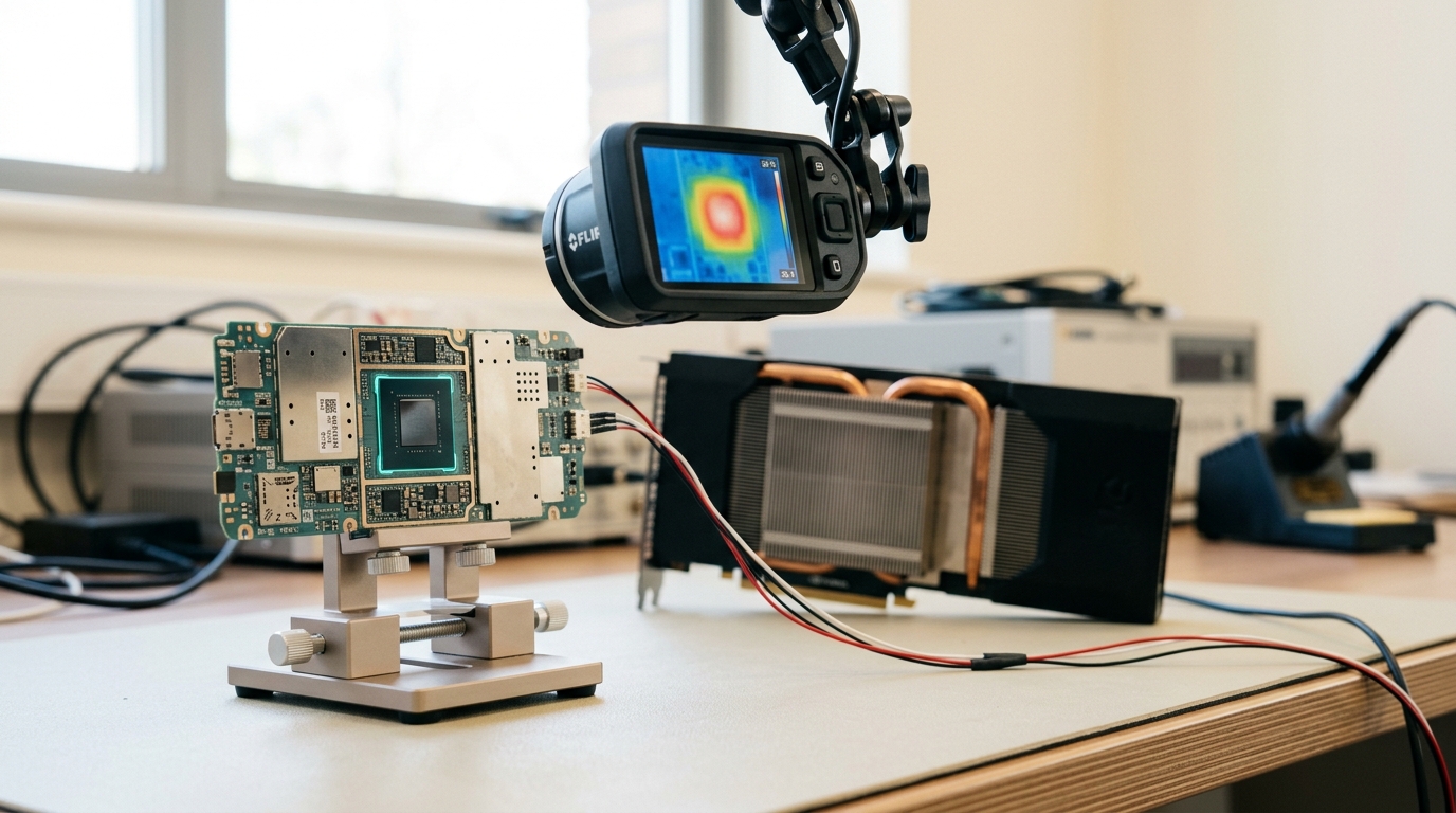
Thermal budget is the wall that arrives late. A sealed handheld device has no fan and a skin-temperature limit imposed by what a hand will tolerate. Peak power is therefore a transient that the thermal mass absorbs for a few seconds, after which the governor caps frequency and the machine settles to whatever it can dissipate indefinitely. Bhat and colleagues, characterising commercial mobile platforms experimentally, put the mechanism plainly: “high performance comes at the expense of larger power density, which leads to higher skin temperatures” ^[5]. The practical consequence for language models is that the number worth measuring is not the first token’s rate but the rate at the tenth minute. A 2026 benchmarking study of small-model inference under sustained load reports that on one flagship handset the device “loses nearly half its throughput within two iterations”, while a low-power dedicated accelerator held 6.9 tokens per second under 2 watts with “near-zero variance”, and a laptop-class discrete GPU sustained 131.7 tokens per second at 34.1 watts ^[6]. Those three numbers are not a ranking of products — they were measured on different hardware classes serving different purposes — but together they make the structural point: on a thermally limited device, sustained and peak are different machines.

Battery energy is the wall the user feels. Energy per query, not latency, determines whether a feature can be invoked casually or must be rationed. And the energy is dominated by data movement rather than by arithmetic. Horowitz’s ISSCC analysis of computing’s energy problem gives the ratio directly: “the energy cost of a DRAM access (1 to 2nJ) is a couple of orders-of-magnitude higher than the cost of an internal cache access or functional operation (10pJ)”, with the off-chip interface alone taking “over 20pJ/bit” ^[2]. That figure is from 2014 and absolute values have improved since, but the ordering has not: fetching a byte from main memory costs far more energy than doing arithmetic on it. This is why the bandwidth wall and the battery wall are the same wall seen from two sides. The bytes that cost you time are the bytes that cost you charge.

Cold start is the wall that is invisible in benchmarks. A served model in a datacentre has its weights resident in accelerator memory across millions of requests; the load cost is amortised to nothing. On a device the model may not be resident at all when the user taps, and the first token includes paging weights from flash. Alizadeh and colleagues addressed this case explicitly, keeping parameters in flash and streaming them in, and reported that windowing and row-column bundling allowed models “up to twice the size of the available DRAM” to run, with inference “4-5x faster” on CPU and “20-25x faster” on GPU than naive loading ^[4]. The technique is impressive; what it reveals is more important. On a device, storage bandwidth has been promoted into the inference path, and a benchmark that reports steady-state tokens per second on a warm model has quietly deleted the part of the latency the user actually experiences.

Why bandwidth binds harder here

The general form of the argument is old and well posed. Williams, Waterman and Patterson built the roofline model on the premise that “for the recent past and foreseeable future, off-chip memory bandwidth will often be the constraining resource”, and defined operational intensity as operations per byte of DRAM traffic ^[1]. Their bound is one line, and it is the single most useful line in this whole subject:

with $R_{\mathrm{peak}}$ the peak arithmetic rate, $B$ the achievable memory bandwidth and $I$ the operational intensity of the kernel. If $I$ is small, the second term wins and the accelerator’s headline throughput is irrelevant.

Autoregressive decoding sits at the far left of that graph. Generating one token requires reading essentially every weight and the accumulated key-value cache once, and performing roughly two arithmetic operations per parameter. At one byte per weight the intensity is about two operations per byte; at four bits per weight, about four. Pope and colleagues formalised this partitioning problem for large transformers and showed how latency, throughput and cost trade off under different sharding strategies, with generation and prefill behaving as different regimes ^[3]. The bound that matters on a device follows immediately: if $W$ bytes of weights and cache must cross the memory bus for each token and the sustained bandwidth is $B$, then the time per token cannot be less than

no matter how fast the arithmetic units are. As an arithmetic illustration with assumed values rather than a measurement of any product: a four-billion-parameter model at four bits per weight is roughly two gigabytes of weights, so a device sustaining fifty gigabytes per second cannot exceed about twenty-five tokens per second, and a device sustaining twenty-five gigabytes per second cannot exceed about twelve. Nothing in the model, the framework or the prompt changes that ceiling. Only fewer bytes or more bandwidth does.

Now the part that is specific to devices, and it is an analytical claim rather than a sourced finding. The datacentre’s principal defence against this bound is unavailable on a phone. A server raises operational intensity by batching: read the weights once, apply them to many users’ tokens simultaneously, and the cost of the weight read is divided across the batch. Batching converts a memory-bound problem into a compute-bound one, and it is the reason server economics improve with load. A device has one user, one conversation, and a batch size of one. The weight read is amortised across nothing. Whatever bandwidth deficit the mobile memory subsystem has relative to a server accelerator is therefore compounded, not merely inherited: the smaller machine is also denied the trick that made the larger machine efficient. Add to this that the same memory bus is contended by the display and the rest of the system, and that bandwidth on a battery is also energy, and the picture is complete.

This reframes what quantisation is for. On a server, low precision is often discussed as a memory-capacity or cost measure. On a device it is primarily a bandwidth and energy intervention: halving the bits per weight halves $W$ in the bound above and halves the bytes crossing the most energy-expensive interface in the system. Meta’s own report on quantised Llama 3.2 models claims “56% in model size”, a “41% average reduction in memory usage” and “2-4x speedup”, with “decode latency improved by 2.5x and prefill latency improved by 4.2x on average” on an Android handset ^[23]. That is a vendor measurement on vendor-chosen hardware and should be treated as a claim; but the direction and rough magnitude are what the bound predicts.

Quantisation, and what it costs where there is less to spend

The mechanics are well established. Gholami and colleagues frame the opportunity clearly: moving from floating-point to low-precision integers of four bits or fewer “holds the potential to reduce the memory footprint and latency by a factor of 16x” ^[7]. Two post-training methods define current practice. GPTQ uses approximate second-order information to quantise weights to “3 or 4 bits per weight, with negligible accuracy degradation”, and can process a 175-billion-parameter model “in approximately four GPU hours” ^[8]. AWQ starts from the observation that “not all weights in an LLM are equally important” and that “protecting only 1% salient weights can greatly reduce quantization error”, scaling channels by activation statistics rather than reconstructing against a calibration set, with a reported speedup of “more than 3x over the Huggingface FP16 implementation on both desktop and mobile GPUs” ^[9]. Dettmers and Zettlemoyer, sweeping over 35,000 experiments across model families from 19M to 176B parameters at 3 to 8 bits, concluded that “4-bit precision is almost universally optimal for total model bits and zero-shot accuracy” ^[10].

Read together, those results are usually taken as a settled licence to ship four-bit weights. Two more recent findings complicate that reading in exactly the regime small on-device models occupy, and this is where the miniature-engineering analogy earns its place: the quantisation step is an absolute quantity of precision removed, and a small part has less precision to give away.

The first complication is about training intensity. Kumar and colleagues, fitting precision-aware scaling laws over 465 pretraining runs, found that “the degradation introduced by post-training quantization increases as models are trained on more data, eventually making additional pretraining data actively harmful” ^[11]. Now note how small models are actually built. Sardana and colleagues showed that anyone anticipating large inference volumes should “train models smaller and longer than Chinchilla-optimal”, and that quality keeps improving as tokens per parameter are pushed “to extreme ranges (up to 10,000)” ^[25]. That advice has been followed: Microsoft’s phi-3-mini is 3.8 billion parameters trained on 3.3 trillion tokens ^[17], a ratio near a thousand tokens per parameter, roughly two orders of magnitude above the compute-optimal recipe. The analytical consequence, offered as inference rather than as a demonstrated result: the very training regime that makes a small model capable is the regime Kumar’s law identifies as most fragile under post-training quantisation. Capability bought by training longer is, on this account, partly bought on credit against the precision budget — which is precisely the budget on-device deployment then wants to spend again. Quantisation-aware training rather than post-training quantisation is the natural response, and it is notable that Meta’s on-device models were produced with quantisation-aware methods rather than a post-hoc conversion ^[23].

The second complication is about what “no accuracy loss” measures. Dutta and colleagues found that “even when the accuracy of baseline and compressed model are similar”, the models differ substantially in behaviour — answers flip from correct to incorrect and back in significant proportion — and that on generative evaluation the compressed models performed “significantly worse than baseline models” despite matched accuracy ^[12]. Aggregate accuracy is a scalar summary of a distribution, and quantisation perturbs the distribution while leaving the summary intact. For a deployment where a user compares today’s answer to yesterday’s on the same question, distributional distance is the thing that matters, and it is not what the benchmark table reports.

The honest summary is that experts do not fully agree here. The quantisation literature reports negligible accuracy degradation at four bits and is right about what it measures; the distributional literature reports meaningful behavioural change at the same bit width and is also right about what it measures. The disagreement is about which metric should govern a shipping decision, not about the underlying numbers.

Distillation, and where the loss lands

Distillation is now the dominant route to capable small models, and the reason is structural rather than fashionable. A small model trained from scratch on raw text must infer everything from a sparse signal — one correct token per position. A small model trained against a larger model’s full output distribution receives a far richer target per position. Hinton, Vinyals and Dean set out the compression idea in 2015, transferring the knowledge of a cumbersome ensemble into a single deployable network ^[13]; the modern survey literature describes an entire ecosystem built on transferring capability from advanced proprietary models into smaller open ones, with data augmentation as the central mechanism ^[14].

The frontier small-model reports now state the method openly. The Gemma 3 technical report describes a family from 1 to 27 billion parameters trained with a distillation-based approach and an improved post-training recipe, and reports that the 4B instruction-tuned model matches the previous generation’s 27B model ^[15]. Architecture matters too, and matters more at small scale than intuition suggests: MobileLLM found that for sub-billion models, architecture — deep-and-thin layouts, embedding sharing, grouped-query attention — drives quality rather than parameter or data quantity alone, reporting a 2.7% and 4.3% accuracy gain over prior 125M and 350M state-of-the-art models ^[18].

Where does the loss land? The most useful frame available is capacity. Allen-Zhu and Li estimate that language models “can and only can store 2 bits of knowledge per parameter, even when quantized to int8” ^[19]. If that estimate is even approximately right, it partitions what distillation can and cannot carry. Style, format, instruction-following, refusal behaviour, tool-call syntax and the general shape of good reasoning are policies — they are cheap in parameters and transfer well. The long tail of specific facts is storage, it is bounded by parameter count, and it cannot be transferred into a body that has no room for it. This is why a well-distilled 4B model can feel indistinguishable from a frontier model on a formatting or summarisation task and then fail flatly on an obscure factual question: the part that transferred was the behaviour, and the part that did not was the contents.

It also explains why retrieval and tool use are not optional add-ons on device but load-bearing architecture. If capacity is the binding limit on stored knowledge, then supplying knowledge at inference time is the only route around it that does not require a larger model.

The advantages that are not about cost

On-device inference is usually justified by unit economics. That is the least interesting reason, and it is contingent — server prices fall. Four advantages are structural and do not depend on the cost curve.

Privacy as an architectural property. When data never leaves the device there is no server-side breach surface to reason about. Apple’s Private Cloud Compute documentation states the underlying comparison explicitly, noting that data on-device avoids “any centralized point of attack” while server processing “requires unencrypted access to the user’s request and accompanying personal data” ^[21]. Google’s Android documentation makes the same argument for Gemini Nano running in the AICore system service, stating that it “doesn’t store any record of the input data or the resulting outputs after processing” and that AICore “does not have direct internet access” ^[22]. Both are vendor claims about vendor systems and are not independently verified here. The point that survives regardless of whose claim you credit is the difference in kind: a policy promise about server-side data handling and the absence of a server are not the same guarantee, and only one of them is auditable by not being there.

Offline operation. A device model works on an aircraft, in a tunnel, in a hospital basement, in a country the vendor does not serve, and during the vendor’s outage. Google’s documentation puts this among the primary reasons for the design, stating that Gemini Nano “lets you deliver rich generative AI experiences without needing a network connection” ^[22]. For consumer convenience features this is a nicety. For anything safety-adjacent it is the whole requirement, because a feature that fails when connectivity fails is a feature that fails exactly when conditions are bad.

A latency floor you own. Round-trip network time is a distribution with a long tail that no amount of server optimisation removes. On-device inference replaces a variable network term with a fixed local one. The floor may be higher in the median case and it is nearly always lower in the tail, and for interactive interface behaviour — inline suggestion, live transcription, on-type rewriting — tail latency is what users perceive as responsiveness.

Independence from a release schedule. A pinned local model is a frozen artefact. It does not change on a Tuesday because a provider promoted a new version behind an alias, and its behaviour under your prompts on your evaluation set is a property you control. Apple’s account of its on-device foundation model describes roughly a three-billion-parameter model designed to run efficiently on devices alongside a larger server model ^[20]; whatever one thinks of the capability trade, the deployment property is real. For regulated workflows where a validated system must remain the validated system, this is often the deciding argument and has nothing to do with price.

The hybrid boundary, and why it is hard

Almost every shipping system is hybrid: a small model handles most requests and hands the rest to a server. Routing between a weak and a strong model is an active research area, and RouteLLM reports that routers trained on human preference data can cut cost “by over 2 times in certain cases” without compromising response quality, with the learned routers transferring even when the underlying models are swapped ^[24]. That work was done in a server context where both models are reachable at the same latency and the only cost is money. The device boundary is harder for four reasons that do not appear in that setting.

The decision precedes the evidence. Whether a request needs the larger model is a fact about the answer, and the router must decide before the answer exists. Any signal cheap enough to compute on-device is, by construction, a weak proxy for a property that would take the full computation to establish.

Escalation is not free — it is additive. If the local model attempts the request and then defers, the user pays local latency plus network latency plus server latency. A router that is wrong in the conservative direction wastes money; a router that is wrong in the optimistic direction wastes the user’s time twice.

The routing decision is itself a disclosure. If the device escalates only sensitive or unusual queries, the act of escalation leaks the classification even when the payload is protected. A privacy architecture built on “we only send the hard ones” has made the decision to send into a signal.

Context must cross the boundary too. A conversation held locally has local state. Escalating mid-conversation means transmitting the history that made the request answerable, which is exactly the material the local execution was protecting, and reconstructing state on the server that the device already held.

The design that avoids most of this is not a router at all but a capability split: assign whole classes of task to the device permanently — transcription, rewriting, classification, extraction, on-device retrieval — and reserve the server for classes that are known in advance to need it, with an offline fallback for every one of them. That trades some average quality for a boundary that is stable, explicable to users, and does not leak through its own decisions. Apple’s published architecture, pairing an on-device model with a separate server tier, is consistent with that split ^{[20, 21]}, though the routing policy itself is not disclosed.

What small models still cannot do

Three limits are structural, not temporary.

Long-tail knowledge. If storage is bounded by parameters at roughly the rate Allen-Zhu and Li estimate ^[19], a model that fits in two gigabytes cannot hold what a model of twenty times the size holds, and no distillation recipe changes that arithmetic. It can be routed around with retrieval; it cannot be trained away.

Long context. Attention state grows with sequence length, and on a device it grows into memory that is already the binding constraint. This is why context handling appears as an architecture decision in small-model reports rather than a configuration flag: Gemma 3 reduced key-value cache overhead by increasing the ratio of local to global attention layers and keeping local spans short ^[15]. Long context on device is paid for in the currency that is scarcest.

Deliberation. This is the sharpest inversion in the whole subject. The most reliable modern route to harder reasoning is to spend more computation at inference time — more tokens, more attempts, more search. In a datacentre that compute is available on demand and is charged for. On a battery-powered, thermally capped device it is the single most expensive thing you can do, because energy per query scales with tokens generated:

with mean power $\bar{P}$, tokens generated $N_{\mathrm{tok}}$ and sustained token rate $r$. Both $\bar{P}$ and $r$ are set by the thermal wall, and $r$ falls as the device heats — so a long deliberation is charged at a worsening exchange rate the longer it runs, which is exactly the behaviour the sustained-load measurements show ^{[6, 5]}. The remedy that works best in the cloud is the one the device can least afford. Any claim that a small model closes a reasoning gap by thinking longer needs to be checked against the device’s sustained rate, not its first-token rate.

Predictions, with the observations that would falsify them

These are forecasts, separated from the sourced analysis above. Horizon: 8 August 2028. They assume no discontinuity in memory technology reaching consumer devices and no regulatory mandate forcing local processing.

One. On-device model reporting will shift from parameter count to a residency-and-bandwidth figure — effective memory footprint plus sustained tokens per second after a stated warm-up — because parameter count has stopped predicting anything a user experiences. Indicator: vendor model cards leading with footprint and sustained rate. Disconfirmed if published on-device specifications in 2028 still headline parameter count with no sustained-throughput disclosure.

Two. Quantisation-aware training will displace post-training quantisation as the default for models shipped to devices, driven by the interaction between extreme token-per-parameter training and post-hoc precision loss. Indicator: small-model technical reports describing low-precision training rather than a conversion step. Disconfirmed if leading on-device releases in 2028 are still produced by post-training conversion of a full-precision checkpoint.

Three. The device-cloud boundary will settle on capability splits rather than per-request quality routers in consumer products, because the routing decision’s own leakage and its additive latency are harder to fix than its cost is to pay. Disconfirmed if major consumer platforms ship user-visible per-request escalation driven by a learned difficulty predictor.

Four. Evaluation of on-device models will acquire a thermal axis: results reported at a stated duration under sustained load, not at first token. Disconfirmed if the standard on-device benchmarks of 2028 still report only warm steady-state or single-shot throughput.

None of these requires a capability breakthrough. They follow from the envelope already described.

What to take away

Building a model for a device is model engineering in the literal sense. The mechanism is the same one, and it is being reproduced at a fraction of the scale, and the tolerances do not shrink in proportion: the precision you remove by quantisation is an absolute amount, and a smaller model has less of it to spare. Some features cannot be reproduced at all — the long tail of stored knowledge, an unbounded context, and long deliberation on a battery — and the competent response is to design around their absence rather than to pretend the miniature is the full-size machine.

Ask, in order: what is resident, how many bytes cross the bus per token, what the device sustains after ten minutes, what a query costs in charge, and what happens when there is no network. If a claim about an on-device model does not answer those five, it is describing a benchmark, not a deployment.