How Mathematics, Proof, and Scientific Computation Actually Work

Three machines, one discipline

A proof assistant checking a theorem, a weather model advancing one more timestep, and a CT scanner turning detector counts into a cross-section look like unrelated pieces of software. They are the same discipline wearing different clothes. In each case a claim must be produced from something less than certainty — a chain of inference too long for a person to check by eye, a physical process too chaotic to track exactly, a measurement too incomplete to determine a unique answer — and in each case there is a precise, checkable account of how much the machine can be trusted and where that trust runs out.

This article opens a series on mathematics, proof, and scientific computation, and it starts by building the mechanics from the ground rather than starting from headline results. Three mechanisms carry the argument: how a formal proof assistant such as Lean or Coq actually reduces a mathematical argument to something a small, auditable kernel can check line by line; how floating-point rounding error is generated and bounded as a numerical simulation runs; and how an inverse problem such as tomographic reconstruction is made solvable at all through regularization. A fourth thread — machine-assisted mathematics and uncertainty quantification — runs through all three, because increasingly none of them is done by a single deterministic run.

Throughout, four registers are kept apart deliberately. Fact: a specific theorem was checked by a specific kernel, a specific error bound was proved for a specific algorithm. Vendor or project claim: a tool’s own description of what it accomplishes. Analysis: what a result does and does not license as a conclusion. Scenario or prediction: what might follow, stated with a horizon and a way to know if it didn’t happen. Mathematics is unusually good at making this separation crisp, because a proof either checks or it doesn’t — but the surrounding claims about what a checked proof means are not themselves proofs, and are treated that way here.

What a formal proof assistant is actually checking

A textbook proof is written for a human reader who fills gaps with background knowledge, intuition, and trust in the author. A formal proof, in a system such as Lean or Coq, is written for a small program called the kernel, which accepts nothing on trust. Every inference step must be an instance of one of a short list of primitive rules in the system’s underlying logic — typically some variant of type theory — and the kernel’s only job is to check that each step really is such an instance.

This split between kernel and everything else is the single most important design fact about a proof assistant, and it is why formal proofs are trustworthy in a way that “the computer checked it” alone would not be. Most of a modern proof assistant’s code is not trusted: elaborate tactic engines search for proofs, automation fills in routine steps, and a large standard library of previously proved lemmas is assembled by a whole community. None of that machinery has to be correct for the final result to be correct, because all of it, however it was produced, ultimately emits a low-level proof term or a sequence of kernel calls, and it is only that output the kernel checks. De Moura and Ullrich’s description of the Lean 4 kernel makes this “small trusted core, large untrusted elaborator” architecture explicit as the system’s central trust boundary ^[4].

This is why two of the most-cited events in formal mathematics are not about new theorems so much as about closing exactly this trust gap on an old one. Appel and Haken’s 1976 proof of the four-color theorem was controversial for over a decade because part of the argument was an exhaustive case check performed by an unverified computer program — a human referee could not check it directly, and had to trust the program instead of the mathematics. Georges Gonthier’s 2008 formalization, carried out in the Coq proof assistant, redid the entire argument, including the combinatorial case analysis, as a sequence of kernel-checked steps, so that the residual trust was moved from “trust this specific unverified C program” to “trust the much smaller, much more scrutinized proof kernel” ^[1]. The mathematical content did not change; what changed was the size and character of the thing a skeptic has to trust.

The Flyspeck project’s formal proof of the Kepler conjecture — that no packing of equal spheres in three-dimensional space is denser than the familiar face-centered cubic and hexagonal close arrangements — followed a similar arc for a harder reason. Thomas Hales’s original 1998 proof combined conventional argument with large-scale numerical optimization over thousands of cases, and referees explicitly could not certify the numerical part with full confidence after years of review. The Flyspeck team spent roughly a decade re-deriving the entire argument in the HOL Light and Isabelle proof assistants, reducing both the combinatorics and the numerical inequalities to kernel-checked steps, and published the completed formalization in 2017 ^[2]. That a proof combining discrete case analysis with continuous nonlinear optimization could be pushed all the way to a machine-checked certificate is itself the noteworthy fact — it demonstrates a mechanism, not a shortcut past the underlying mathematics.

None of this makes proof assistants a substitute for mathematical understanding. A kernel check certifies that a specific chain of primitive steps is valid; it says nothing about whether the theorem statement means what a reader thinks it means, whether the formalization actually captures the informal claim it is meant to represent, or whether the proof illuminates why the result is true. Formalizing the classical statement of a theorem incorrectly and then proving that incorrect statement is a documented failure mode, distinct from — and in some ways more insidious than — an unchecked gap in an informal proof, because it produces a green checkmark. The kernel’s guarantee is narrow and absolute within its scope; the scope itself still depends on human judgment.

Building the library the checking runs against

An individual kernel-checked theorem is not useful in isolation; formal mathematics needs a shared library of previously proved results the way ordinary mathematics needs a shared literature. Lean’s mathlib is the largest such effort in that ecosystem: a single, continuously maintained library covering large parts of undergraduate and graduate mathematics — algebra, analysis, topology, measure theory, number theory — built collaboratively so that a new formal proof can cite existing formalized lemmas rather than re-deriving elementary facts from primitives every time ^[3].

This is where the “goal state” a working mathematician actually watches lives. At each point in an interactive proof, the assistant displays the current set of open subgoals — what remains to be shown, given what has already been established and which hypotheses are in scope. Writing a formal proof, in practice, is an iterative loop of applying a tactic, watching the goal panel update, and repeating until no subgoals remain; the kernel’s replay of the resulting low-level proof term is what finally certifies the whole chain, but the interactive goal state is the interface through which a person actually does the work. A large shared library changes the economics of that loop enormously: a step that would require deriving a fact from raw axioms instead becomes a single call to an already-checked lemma, at the cost of a genuine engineering burden — a library of this scale needs its own maintenance discipline, deprecation process, and review culture, mirroring an ordinary software codebase as much as it mirrors a body of mathematics.

Floating-point arithmetic never gives an exact answer, by design

Move from formal proof to numerical simulation and the trust problem inverts. A proof assistant’s kernel is exact but slow to reach; a floating-point simulation is fast but never exact, and the discipline is about bounding how inexact it is allowed to become.

Computers represent real numbers with a finite number of bits, following a specification — IEEE 754 — that fixes the format and the rounding behavior of arithmetic exactly enough that different compliant hardware and software give reproducible results for the same operations ^[5]. The standard’s core guarantee is deceptively narrow: each individual elementary operation is correctly rounded, meaning the result is the closest representable floating-point number to the true mathematical result of that one operation. For a single addition or multiplication, this means

where $u$ is the unit roundoff — roughly $10^{-16}$ for standard double precision — and $\mathrm{op}$ is addition, subtraction, multiplication, or division. Each single step, in other words, is correct up to a tiny, precisely bounded relative error.

The difficulty is that a simulation is not one operation; it is billions of them, composed. A relative error of $u$ per operation does not by itself say anything about the error after a million timesteps, because errors can compound, cancel, or amplify depending entirely on the structure of the calculation. This is the subject of rounding error analysis, and it produces two genuinely different kinds of statement that are often conflated in casual discussion. A forward error bound asks how far the computed answer can be from the true answer. A backward error bound asks, instead, how large a perturbation of the original input would have been needed to produce the computed output exactly — and it is frequently the more tractable and more informative quantity, because it separates the algorithm’s behavior from the problem’s own sensitivity. Higham’s systematic treatment of this distinction, and of the perturbation theory needed to convert a backward bound into a usable forward bound, is the standard reference for how these bounds are actually derived and what they do and do not promise ^[6].

That distinction is what separates an algorithm’s fault from a problem’s fault. A problem’s intrinsic sensitivity to input perturbation is measured by its condition number: a well-conditioned problem, computed by a numerically stable algorithm, yields a small forward error because both factors are small; a well-conditioned problem computed by an unstable algorithm can still yield a large forward error, because instability amplifies an already-small backward error into an unacceptable one. Conversely, no algorithm — however carefully implemented — can produce a reliably accurate answer to an intrinsically ill-conditioned problem, because tiny, unavoidable input rounding is already enough to move the true answer substantially. Diagnosing a simulation’s numerical trouble means asking, separately, whether the underlying continuous problem is sensitive and whether the discrete algorithm computing it introduces additional instability beyond that sensitivity — collapsing the two into a single “it’s just rounding error” is the most common way this kind of trouble gets misdiagnosed.

Long-running simulations — climate models, molecular dynamics, orbital mechanics — add a further wrinkle: chaotic sensitivity to initial conditions means that even an idealized, exact calculation would diverge exponentially from a calculation started from a microscopically perturbed initial state. In that regime, a floating-point simulation’s own rounding error acts as exactly such a perturbation, and no increase in numerical precision removes the divergence; it only delays, by a bounded number of Lyapunov timescales, the point at which two runs starting from bitwise-identical inputs but computed with different operation orderings (as happens routinely under parallel execution) stop resembling each other. This is a fact about the underlying dynamical system, not a defect in the arithmetic, and it is why single deterministic runs of chaotic models are supplemented with ensembles of perturbed runs rather than trusted individually — a point this article returns to below.

Inverse problems: recovering a cause from an incomplete effect

The third mechanism runs in the opposite direction from simulation. A simulation starts from a known model and known initial conditions and computes forward to a prediction. An inverse problem starts from an observed effect and asks what cause produced it — and the honest answer, for most real measurement setups, is that many different causes are consistent with the data actually collected.

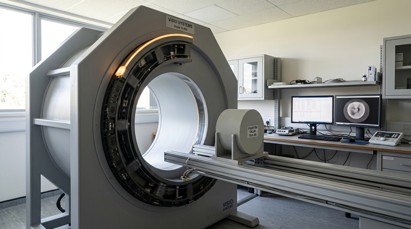
Tomographic reconstruction is the clearest physical example. A computed tomography scanner does not measure the interior structure of an object directly; it measures a finite set of line-integral projections — how much a beam was attenuated along many straight paths through the object, taken from many angles around it — and the reconstruction problem is to recover the two- or three-dimensional attenuation map consistent with those projections. Classical algebraic reconstruction methods set this up explicitly as a large system of linear equations, one per measured ray, and solve it iteratively; Gordon, Bender, and Herman’s 1970 algebraic reconstruction technique (ART) for electron microscopy and X-ray photography was among the first to frame three-dimensional reconstruction from projections this way computationally, rather than through the continuous Radon-transform inversion formulas developed earlier in pure mathematics ^[8].

The trouble is that with a finite number of projection angles and a finite detector resolution, the resulting linear system is underdetermined and ill-conditioned: many attenuation maps fit the measured data equally well within noise, and small measurement noise can be amplified into large, structured artifacts in a naively reconstructed image. This is the general signature of an ill-posed inverse problem in the sense formalized by Hadamard — a solution may fail to exist, fail to be unique, or fail to depend continuously on the data — and tomography exhibits the second and third failure modes acutely.

Regularization is the standard mathematical answer: instead of solving the raw, ill-conditioned system, one solves a modified problem that trades a small, controlled amount of bias for a large reduction in the amplification of noise. Tikhonov regularization is the paradigmatic form, replacing the bare least-squares fit with a penalized objective

where $A$ is the forward projection operator, $b$ the measured data, $L$ a penalty operator (often favoring smoothness), and $\lambda > 0$ a regularization parameter controlling the trade-off. As $\lambda \to 0$ the solution approaches the raw, noise-amplifying least-squares fit; as $\lambda$ grows the solution becomes smoother and more stable but increasingly biased away from the true structure. Neubauer’s analysis of Tikhonov regularization for nonlinear ill-posed problems established the convergence-rate theory that tells a practitioner how the regularization parameter should shrink as data quality improves in order for the regularized solution to actually converge to the true one, rather than converging to a fixed, permanently biased answer ^[9]. Choosing $\lambda$ well — commonly via the discrepancy principle or an L-curve criterion — is itself a nontrivial estimation problem, and a poorly chosen $\lambda$ can quietly produce a smooth, plausible-looking, and wrong reconstruction.

A related and more recent development, compressed sensing, showed that when the true underlying signal or image is known in advance to be sparse in some representation — few nonzero wavelet coefficients, for instance — it can sometimes be recovered exactly from far fewer measurements than classical sampling theory would require, provided the measurement process satisfies certain incoherence conditions. Candès, Romberg, and Tao’s foundational analysis established the precise conditions and error bounds under which this recovery is possible ^[7]. This result is properly read as a statement about a specific class of signals and measurement operators, not a general repeal of the data requirements for reconstruction; it does not apply to arbitrary images, and its guarantees depend on incoherence properties that must be checked for the actual acquisition system, not assumed.

Where the three mechanisms meet: machine-assisted, uncertainty-aware mathematics

These three mechanisms increasingly do not run in isolation. Large numerical simulations are used to search for counterexamples or verify special cases that feed into formally checked proofs, as happened in parts of the Flyspeck effort. Formal methods are beginning to be applied to floating-point arithmetic itself, proving bounds on rounding error for specific numerical kernels with the same kernel-checked rigor used for pure-mathematics theorems. And inverse-problem reconstructions are validated, in practice, not by a single deterministic solve but by ensembles: many reconstructions run from perturbed or resampled data, whose spread indicates how much of the answer is actually supported by the measurements rather than by the choice of regularization parameter or numerical method.

This ensemble discipline is the practical answer to a question raised earlier: since a single floating-point run cannot distinguish a genuinely uncertain physical quantity from an artifact of one particular rounding path or one particular regularization choice, uncertainty quantification runs many variants — perturbed initial conditions, perturbed data, different but equally defensible regularization parameters — and reports the resulting spread as an estimate of how much confidence the final number deserves. This is analysis, not a guaranteed bound in the way a kernel check or a proven error bound is: the spread across an ensemble is only as trustworthy as the ensemble’s coverage of the actual sources of uncertainty, and a poorly designed ensemble can understate uncertainty just as easily as a single run can hide it.

A scenario, stated as such and not as fact: if kernel-checked formal methods continue to reduce their manual formalization cost — through better automation for translating informal mathematical statements and proof search — a plausible five-to-ten-year development is that formally verified numerical error bounds become a standard, checked artifact accompanying safety-critical simulation code, the way unit tests are standard today. The observable indicator would be a measurable rise in published formally verified numerical kernels in that period; the disconfirmation condition is straightforward — if formalization effort per verified numerical result does not fall substantially from where it stands today, this adoption will not happen on that timescale, because the cost will continue to exceed what most simulation projects can justify.

What actually changed and what did not

None of the three mechanisms described here replaces mathematical judgment with mechanical certainty across the board. A kernel check certifies a chain of primitive inferences, not that the formalized statement captures the intended informal claim. A rounding-error bound certifies what a specific algorithm does to a specific well- or ill-conditioned problem, not that a simulation’s physical model itself is correct. A regularized reconstruction certifies a bias–stability trade-off given assumptions about the true signal’s structure, not a unique, assumption-free recovery of ground truth. In each case, formal or numerical rigor narrows a large space of uncertainty to a small, precisely characterized remainder — and the discipline consists exactly of knowing where that remainder still is.