How AI for Science and Medicine Actually Works

Four problems, one shared shape

Say “AI for science” and the mental image is usually a chart: a benchmark score climbing, a discovery counted, a diagnosis confirmed. That is the wrong level to look at if the question is how these systems actually work. AlphaFold’s Evoformer, GNoME’s crystal-graph networks, GraphCast’s mesh, and an FDA-cleared radiology model were built by four different teams, for four different sciences, on four different kinds of data, and they do not descend from one another. Yet opened up, they share a recognisable shape: a structured representation of the domain’s own data, a network trained to operate on that representation, and — in every case that has actually changed a field — a loop that closes the network’s output against an independent, physical ground truth.

This article stays at that level. It is not a survey of what these systems have achieved, not an assessment of how well validated they are, and not an argument about where the field is heading — those are separate questions, treated separately elsewhere. Here the question is narrower and more mechanical: given a sequence, a chemical-composition space, a grid of atmospheric variables, or a medical scan, what computation actually happens between input and output, and what did the network see during training that makes that computation possible.

Four systems carry the argument. AlphaFold2 and AlphaFold3, for protein structure. GNoME and the A-Lab, for materials discovery. GraphCast, for medium-range weather forecasting. And the architecture common to FDA-cleared diagnostic imaging models, illustrated through LumineticsCore, the first autonomous AI diagnostic system the FDA authorised. Each section below opens one system’s actual computation; a closing section names what is structurally common to all four, and where that commonality stops.

Protein structure: what the Evoformer reads, and what diffusion changed

A folded protein is a molecule that has settled, out of an astronomical number of possible configurations, into one shape determined by its amino-acid sequence. Predicting that shape from the sequence alone was, for decades, treated as a search problem: try candidate conformations, score them against a physics-based energy function, and hope the search finds the true minimum. AlphaFold2 replaced the search with a different kind of computation, and the paper describing it — published in Nature in 2021 by John Jumper and colleagues at DeepMind — is unusually explicit about the architecture, down to block counts and array shapes ^[1].

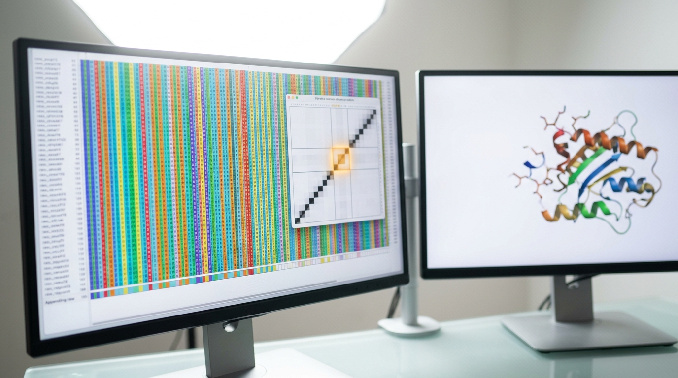
The input is not the raw sequence alone. It is a multiple sequence alignment, a matrix in which each row is a homologous sequence found in public databases and each column is a position in the target protein, aligned so that corresponding residues line up across rows. Positions that co-vary across many organisms — where a substitution at one site is consistently accompanied by a compensating substitution at another — carry information about which residues sit physically close in the folded structure, even though the alignment itself says nothing about geometry. That coevolutionary signal, not any stored lookup of known structures, is the primary evidence the network reasons over. Where structures of related proteins are available, the network also accepts them directly as templates: three-dimensional atomic coordinates of homologous structures, folded in as an additional, more direct source of geometric evidence ^[1].

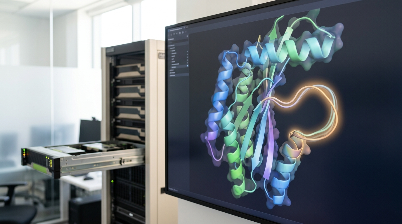
Both are processed by the Evoformer, a stack of forty-eight blocks that maintain two representations simultaneously and update each from the other. One is the sequence-alignment array itself — sequences by residues — refined through row-wise and column-wise attention. The other is a pairwise array, residues by residues, representing how confidently the network currently believes any two positions are related in the final structure. The pairwise array is updated through what the paper calls triangle multiplicative updates and triangle self-attention: operations that treat any three residues as a triangle and constrain the edge between two of them using information about their shared relationships to the third, which is one way of building a soft, learned analogue of the geometric consistency a real folded chain must obey. Across forty-eight blocks and up to four cycles of recycling the whole computation back through itself, the pairwise array accumulates from a nearly uninformative starting point into something that behaves like a distance and orientation map ^[1].

The final stage, the Structure Module, is where the pairwise array becomes actual coordinates. It represents each residue’s local frame as a rotation and a translation, and refines these iteratively using a mechanism called Invariant Point Attention — attention computed in a way that does not change if the whole structure is rotated or translated, which matters because a folded protein has no privileged orientation in space. The output is a full set of atomic coordinates, along with the network’s own per-residue confidence in them ^[1].

AlphaFold3, published in Nature in 2024 by Josh Abramson and colleagues, keeps the general two-stage shape — process a representation, then generate coordinates — but changes both stages substantially, and extends the target from single protein chains to complexes involving proteins, nucleic acids, small molecules, ions, and modified residues predicted jointly. The Evoformer is replaced by a simpler Pairformer module that processes only pair and single representations rather than retaining the full sequence-alignment array throughout; multiple-sequence-alignment information is folded into the pair representation early rather than carried forward block by block. Despite that simplification, the dependence on alignment depth persists: proteins with shallow alignments — few known relatives — are still predicted with lower accuracy, which is direct evidence that the coevolutionary signal is still doing real work, not merely convenient scaffolding for the earlier architecture ^[2].

The larger change is in how coordinates are produced. Rather than a Structure Module built on rotations and translations, AlphaFold3 uses a diffusion module that operates directly on raw atom coordinates and a coarse token representation, without rotational frames at all. Diffusion models are trained on a simple, general task: take a true data point, corrupt it with noise at a known level, and train a network to recover the original from the corrupted version. For coordinates $x_0$ noised to $x_t$ at noise level $t$,

with $\epsilon$ drawn from a standard normal distribution and $f_\theta$ the trained network. Generating a structure then means starting from coordinates that are almost pure noise and repeatedly applying the trained denoiser, each pass nudging the atoms closer to a physically coherent arrangement, across many scales at once — from the local geometry of a single ring to the global fold of an entire complex ^[2]. Both AlphaFold2 and AlphaFold3 were trained on structures deposited in the Protein Data Bank; AlphaFold3’s training data was cut at structures released before 30 September 2021, supplemented by sequence databases including UniRef90, Uniclust30, and BFD, and RNA-specific databases including Rfam and RNAcentral ^[2].

Materials discovery: two ways to propose a crystal, one way to check it

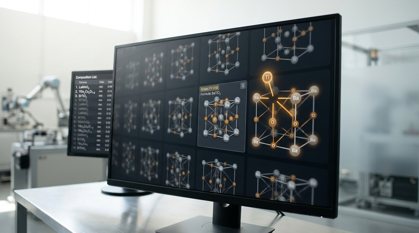
Predicting whether a hypothetical arrangement of atoms would form a stable crystal is a different problem from folding a known chain, because there is no single sequence to condition on — the space of candidate compositions and lattice geometries is, in principle, unbounded. GNoME — Graph Networks for Materials Exploration, described by Amil Merchant and colleagues at Google DeepMind in a 2023 Nature paper — addresses this with a graph neural network trained to predict a candidate crystal’s thermodynamic stability directly from its structure, represented as a graph in which atoms are nodes and their bonds are edges ^[3].

The candidates themselves come from two separate generation pipelines rather than one. A structural pipeline takes known crystal structures and substitutes different elements into their lattice positions, testing whether chemically similar substitutions preserve stability. A compositional pipeline proposes candidates from randomised chemical formulas without starting from any known structure at all, reaching into combinations a chemist working from precedent would be unlikely to try. Both streams of candidates are scored by the same graph network for predicted stability, and the highest-confidence predictions are checked against density-functional-theory calculations — an independent, physics-based computational method, expensive per compound but not dependent on the network’s own judgment. Results from that checking step are then folded back into the training set for the next round, an active-learning loop that DeepMind reports raised the network’s precision at identifying genuinely stable materials from around fifty percent to around eighty percent over successive rounds. The completed search identified roughly 2.2 million candidate structures, of which some 380,000 were assessed as sufficiently stable to be plausible synthesis targets ^[3].

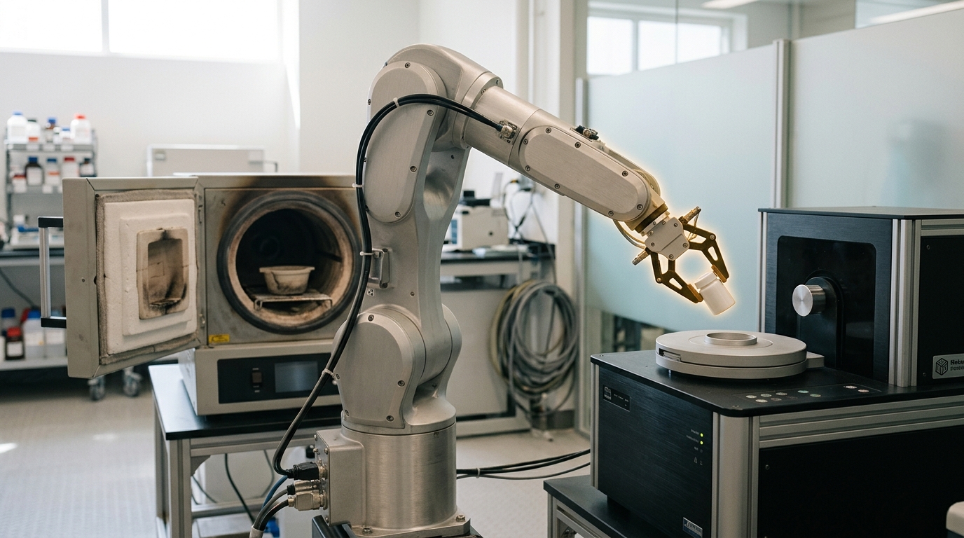
A stability prediction, however confident, is a computational claim about a hypothetical arrangement of atoms — it is not yet a material anyone can hold. Closing that gap is what the A-Lab, described by Nathan Szymanski and colleagues at Lawrence Berkeley National Laboratory and UC Berkeley in a companion 2023 Nature paper, was built to do. A-Lab is a robotic laboratory for solid-state synthesis that chains together computation, literature-derived reasoning, and physical experimentation in one continuously operating loop. Candidate compounds — drawn from large-scale stability data including GNoME’s predictions and the Materials Project database — are handed to a system that proposes synthesis recipes by drawing on patterns extracted from published literature describing how chemically related compounds have previously been synthesised. Robots then execute those recipes: dispensing precursor powders, running solid-state reactions in furnaces, and handing the resulting product to an X-ray diffractometer for characterisation. The diffraction pattern either confirms the target phase formed or reveals what formed instead, and either outcome updates a thermodynamics-grounded active-learning model that revises the next attempt’s recipe. Over seventeen days of continuous, unattended operation, the system worked through dozens of computationally predicted target compounds, adjusting its own synthesis strategy between attempts based on what the diffractometer actually reported rather than what the phase-stability calculation had predicted ^[4].

The two systems are worth holding side by side precisely because they occupy different positions in the same pipeline. GNoME’s graph network never touches a physical sample; its output is a ranked, computational hypothesis. A-Lab never proposes a hypothesis of its own; its active-learning loop operates entirely on the gap between a predicted recipe and a measured diffraction pattern. Neither claim is complete without the other — a stability score is not evidence a compound can be made, and a successful synthesis run does not by itself explain why the computation pointed there in the first place.

Weather forecasting: a graph, not a fluid-dynamics solver

Operational numerical weather prediction works by treating the atmosphere as a fluid governed by known physical laws — conservation of mass, momentum, and energy — and integrating those equations forward in time on a three-dimensional computational grid, starting from an estimate of the atmosphere’s current state built by data assimilation, the same general technique used to construct reanalysis datasets. It is an enormous, physically grounded computation, run on some of the largest supercomputers in the world, and it is the method every graph-neural-network weather model is measured against.

GraphCast, described by Remi Lam and colleagues at Google DeepMind in a 2023 paper published in Science, replaces the equation-integration step with a trained graph neural network operating on an encoder–processor–decoder structure. Weather variables at roughly one million points on a 0.25-degree global grid are first encoded onto a spherical mesh; a processor network then updates each mesh node’s representation by passing messages between it and its neighbours, repeated across the mesh’s structure so that information can propagate across the globe within a single forward pass; a decoder then reads the updated mesh back out to the original grid to produce the forecast. In general form, a message-passing update for a node $v$ with neighbours $\mathcal{N}(v)$ looks like

where $h_v^{(k)}$ is node $v$’s representation after $k$ rounds of message passing, $e_{uv}$ is the edge connecting it to neighbour $u$, and $\psi$ and $\phi$ are learned functions — the same general operation GNoME’s crystal-graph network applies to atoms and bonds, applied here to points on a sphere and the physical processes connecting them. GraphCast predicts five surface variables and six atmospheric variables across thirty-seven pressure levels, ten days ahead, at six-hour steps ^[5].

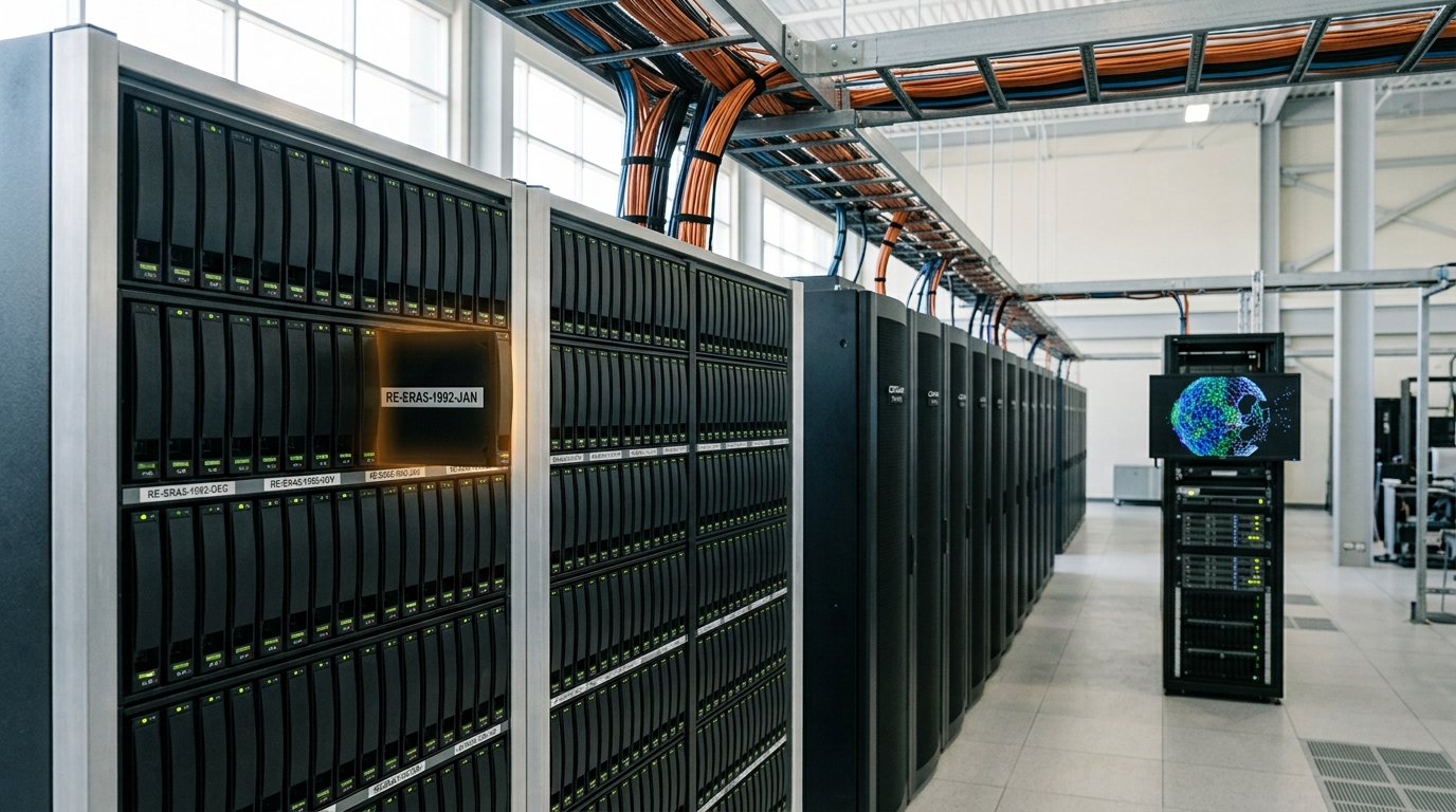
The network is not trained on live observations directly. It is trained on ERA5, the European Centre for Medium-Range Weather Forecasts’ fifth-generation reanalysis product, produced by the Copernicus Climate Change Service. Reanalysis combines historical observations — satellite soundings, radiosondes, surface stations, ship and aircraft reports — with a numerical forecast model through data assimilation, the same technique operational forecasting uses to initialise a fresh run, but applied retrospectively to build a physically consistent, gap-free record of the atmosphere’s past state, in ERA5’s case hourly from 1940 to the present at roughly 31-kilometre resolution ^[7]. Training on four decades of that reconstructed record is what lets GraphCast learn statistical patterns in how the atmosphere actually evolves, without the network itself ever solving a fluid-dynamics equation at inference time. DeepMind reports that a ten-day GraphCast forecast runs in under a minute on a single TPU v4, against the many hours a physics-based run typically takes on a dedicated supercomputer allocation, and that GraphCast forecasts were more accurate than the European Centre’s operational HRES system on ninety percent of 1,380 tested variables and pressure levels ^[6].

The contrast is not “AI versus physics” in any deep sense — the training data GraphCast learns from was itself produced by a physics-based model doing data assimilation. It is a contrast in where the physical reasoning is performed: once, expensively, when ERA5 was built, versus repeatedly, expensively, every time an operational forecast is issued. A trained network amortises that cost, at the price of only being as good, on any given day, as the patterns forty years of reanalysis data managed to encode.

Medical imaging: from a labelled archive to a cleared device

An FDA-cleared diagnostic imaging model is architecturally the least exotic of the four systems here, and that is itself informative. The dominant architecture family is the convolutional neural network — ResNet- and DenseNet-style architectures for classification tasks such as flagging a study as positive or negative for a finding, and U-Net-style architectures for segmentation tasks such as outlining a lesion’s boundary — the same broad family that has driven progress in general computer vision since roughly 2012 ^[10].

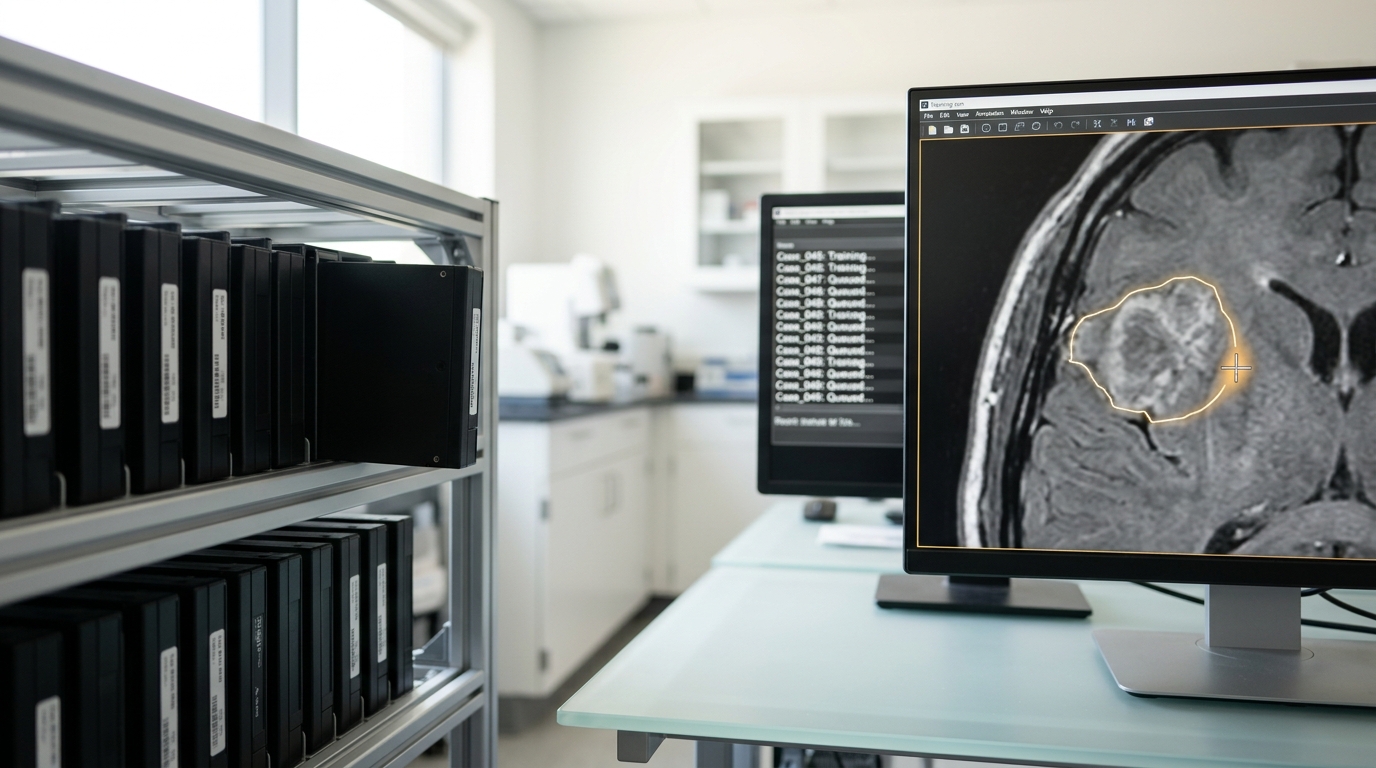
What distinguishes a clinical imaging model is less the network than the data pipeline around it. Training images are extracted from a hospital’s picture archiving and communication system, in DICOM format, and de-identified — protected health information embedded in the DICOM header is stripped before anything is used for training. Ground-truth labels come from expert annotation: a radiologist tracing a segmentation mask around a lesion, or classifying a study according to a diagnostic category, establishing the reference standard the network is trained to reproduce. A typical project splits labelled data into training, validation, and test sets — commonly eighty, ten, and ten percent — or uses cross-validation when the labelled dataset is small, which it very often is, since expert annotation is slow and does not scale the way web-scraped image data does ^[10].

Regulatory clearance in the United States runs predominantly through the FDA’s 510(k) pathway, which authorises a device on the basis of substantial equivalence to an already-cleared predicate device, rather than requiring the ground-up clinical trial a novel drug would need. A systematic review of FDA-authorised AI and machine-learning devices, published in JAMA Network Open in 2025, found 950 such devices authorised through mid-2024, of which 723 — seventy-six percent — were radiology devices; 924 of the full 950, ninety-seven percent, were cleared through 510(k), with 22 through the De Novo pathway for devices with no existing predicate and 4 through full premarket approval. Authorizations accelerated sharply after 2016, reaching 221 in 2023 alone. The same review is candid about a gap: among the 717 radiology devices with reviewable submission documentation, only 33 — five percent — had been evaluated in prospective studies, and only 208 — twenty-nine percent — included any clinical testing at all rather than purely retrospective, algorithm-only performance metrics ^[8]. That gap is a validation question, addressed properly elsewhere in this series; it is noted here only because it is a direct consequence of the 510(k) pathway’s design, and therefore part of how these systems actually reach a reading room, not a separate topic.

One example makes the architecture-to-workflow chain concrete. LumineticsCore, originally cleared as IDx-DR, received FDA De Novo authorisation in April 2018 as the first autonomous AI-based diagnostic system the agency had authorised — autonomous in the specific sense that it issues a diagnostic output without requiring a clinician to separately interpret the underlying image. It analyses fundus photographs captured with a Topcon NW400 retinal camera and classifies a patient as positive or negative for more-than-mild diabetic retinopathy, producing a report with care instructions aligned to American Academy of Ophthalmology practice patterns. Because no ophthalmologist needs to review the image before the result is given to the patient, the device is deployed in primary-care offices, where a technician captures the retinal photographs during a routine visit and the patient receives a result, and any necessary referral, before leaving ^[9]. That workflow placement — inside a primary-care visit rather than a radiology reading room — is only possible because the regulatory clearance covers the full autonomous pipeline, camera to report, not a classifier awaiting a specialist’s sign-off.

The shape underneath, and where it stops applying

Set side by side, the four systems share three structural commitments, in this order. First, domain structure is encoded into the representation before the network sees it — a multiple sequence alignment carries evolutionary constraint, a crystal graph carries bond topology, a spherical mesh carries geographic adjacency, a DICOM series carries calibrated pixel intensities. None of the four networks learns physics or chemistry or geometry from scratch out of raw, unstructured input; each is handed a representation already shaped by what its designers know about the domain. Second, the network itself is a general-purpose pattern learner operating on that representation — attention over a pairwise array, message passing over a graph, convolution over an image grid — with no domain-specific rule about proteins, crystals, or atmospheres hand-coded into its weights. Third, and this is where the four systems diverge most sharply in how rigorously it is applied, the output is checked against an independent, physical ground truth, and that check feeds back into the next round of training or search: density-functional-theory calculations and X-ray diffraction for GNoME and A-Lab, forty years of assimilated observation for GraphCast, expert-annotated scans and — for a cleared device — prospective clinical evaluation for a diagnostic model, and, for a protein, ultimately X-ray crystallography or cryo-electron microscopy on structures the network never saw during training.

That third commitment is also where the analogy runs out, and it is worth being precise about the limit rather than letting it blur. A closed loop against density-functional theory tells you a computed structure is thermodynamically plausible; it does not by itself tell you a robot can synthesise the compound, which is exactly why A-Lab exists as a separate system rather than a claim GNoME could make on its own. A closed loop against forty years of reanalysis tells you a forecasting network has learned real atmospheric statistics; it says comparatively little about how the same network performs on an event structurally unlike anything in its training record — a genuinely novel type of extreme, for instance — because the loop only checks against the past. And a closed loop against retrospective expert labels is not the same evaluation as a closed loop against prospective clinical outcomes, which is precisely the distinction the JAMA Network Open review’s five-percent figure is pointing at. Architecture explains how a system computes its output. It does not, on its own, explain how much that output should be trusted in a specific new case — that is a measurement question, not a mechanism question, and this article has deliberately stayed on the mechanism side of that line.

What follows from the architecture, not from a benchmark

Two forward-looking observations follow reasonably directly from how these systems are built, rather than from any claim about how well they currently perform, and each carries an explicit way it could turn out wrong.

Diffusion-style generation will keep spreading from structure prediction into the generation step of the other three domains. AlphaFold3 already replaced a coordinate-frame-based structure module with a general denoising process; the same operation — corrupt a data point, train a network to reverse the corruption — applies just as naturally to generating candidate crystal structures directly, rather than screening them from two separate hand-designed pipelines the way GNoME currently does, and to generating spatially coherent forecast ensembles rather than single deterministic trajectories. Horizon: by 2029, a leading materials-discovery or ensemble-weather system in active use will use a diffusion or flow-based generative module as its primary candidate- or ensemble-generation step, rather than the discrete substitution-and-random-formula approach GNoME uses today. Disconfirmed if, by that date, the highest-throughput materials-discovery pipelines and the leading operational-weather-ensemble systems are still built primarily on non-generative screening and perturbation methods rather than learned generative models.

The active-learning loop, not the underlying network, will remain the harder engineering problem. GNoME’s stability network and A-Lab’s synthesis planner are each individually well-documented; the harder, less publicised work in both papers is the closed-loop coupling between prediction and physical or computational verification, which is also exactly the piece missing for most of the FDA-cleared imaging devices the JAMA Network Open review examined — a trained network with no prospective feedback loop back to real clinical outcomes. Horizon: by 2029, growth in FDA-cleared imaging devices with documented prospective or human-in-the-loop evaluation will outpace growth in total device authorizations, as closing that loop becomes a competitive and not merely a regulatory consideration. Disconfirmed if the proportion of newly authorised devices with prospective evaluation, as tracked in a successor to the 2025 JAMA Network Open review, stays flat or falls relative to total authorizations over that period.

What “how it works” does and does not answer

None of this is an argument that these four systems are equally mature, equally validated, or equally close to routine deployment — they plainly are not, and the honest accounting of that belongs to the companion pieces in this series that address evidence, benchmarks, and failure modes directly. What this article has tried to do instead is narrower and, for readers trying to evaluate a specific claim about one of these systems, arguably more useful: to make the actual computation legible enough that a claim like “the model predicts protein structure” or “the network forecasts the weather” stops being a black box and starts being a specific, checkable sequence of steps — a representation built from real domain evidence, a network trained to operate on it, and, where the work is furthest along, a loop that closes against something the network cannot simply learn to say the right thing about.