The Bend an Elevator Cannot Fake

A network of optical clocks reports only frequency ratios between its own nodes, and a uniformly accelerating elevator can reproduce any one of those ratios exactly. What it cannot reproduce is derived here and checked against that same elevator.

Revolutionary Life 75, Series D, No. 9 — this article is the paper's summary; the full text (PDF): https://absolutedigitalpublishers.com/papers/revolutionary-life-75-d09-clock-network-curvature.pdf

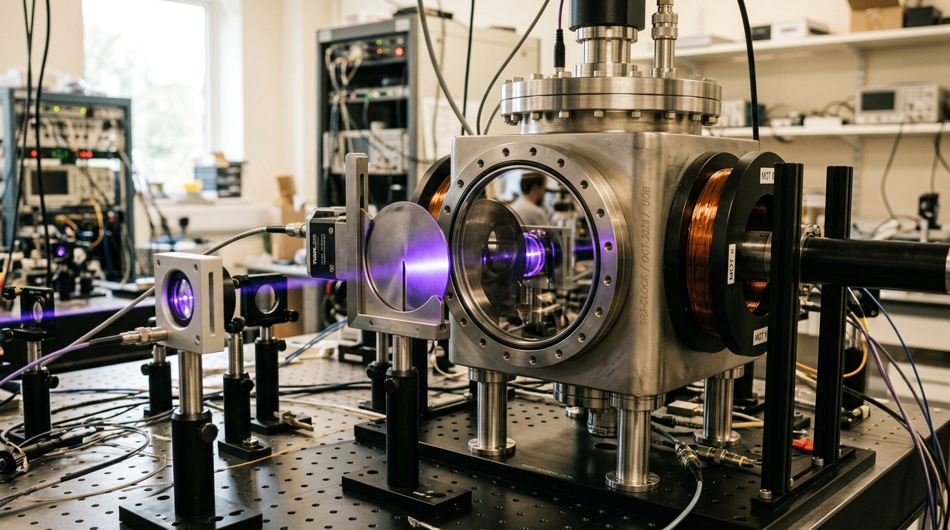
The network's first node: whatever ratio this clock reports, it reports about itself, never about a field it has agreed to share. — Image prompt and art direction by Brecht Corbeel; generation pending.

Abstract

For a network of optical clocks linked by phase-coherent fibre, this article derives two diagnostics from one edge datum, the log frequency ratio between linked clocks: a graph cycle residual from the network's incidence matrix, and a tidal curvature estimator from second differences of the fitted node potential. The cycle residual is proved, as an exact linear-algebra identity, to vanish whenever the data come from any single-valued node potential, curved or flat, so a closed loop audits rotation, drift, and bad links, never curvature by itself. The tidal estimator is derived from the geodesic deviation equation for a static metric that includes the uniformly accelerated case: it vanishes identically there, where the naive second difference does not, and it reduces at weak field to the textbook Newtonian tidal tensor. An exact analytic evaluation using published clock stability finds order-unity sensitivity to Earth's tidal signal needs roughly two hundred metres of vertical separation, a scale already spanned by deployed transportable-clock experiments measuring a different quantity. No simulation ran; the estimator is one stated-frame Riemann component, not a scalar invariant.

The Bend an Elevator Cannot Fake

Two optical lattice clocks sit in two buildings connected by an actively stabilized optical fibre, and once every averaging interval the comparison electronics writes down a single number: the ratio of their frequencies. That number is real, repeatable, and, by itself, silent. It cannot say whether the two clocks disagree because one building sits on a denser slab of foundation rock, because the hill it stands on is honestly higher in a gravitational potential a spirit level could also certify, or because spacetime is genuinely bent between them in a way no single pair of clocks could ever expose on its own. The comparison hands over a ratio; the physics has to be supplied afterward, by construction — and the construction can go wrong in one specific, checkable way that this article derives rather than assumes.

Neither clock in that comparison has ever seen the other. Each keeps a transition frequency locked by its own vacuum chamber, its own lasers, its own magnetic shielding; the only thing that ever crosses the fibre between them is a phase, compared continuously rather than exchanged as a stamped timestamp. That distinction — a running phase comparison rather than a one-off time transfer — is precisely what makes the ratio meaningful in the first place, and precisely what later sections have to be careful never to contaminate with an unmodelled path effect.

The derivation keeps to a strict boundary. Nothing below introduces a new field, a new force, or a revised metric. Every equation either restates general relativity as it already stands or restates ordinary linear algebra applied to a graph of clocks. The claim on trial is narrower than “clocks feel gravity,” which nobody disputes, and for that reason it is more useful: that one specific, exactly derived combination of a clock network’s own frequency ratios is a genuine, stated-frame component of the Riemann curvature tensor, that a different and equally natural-looking combination is not curvature at all no matter how large it grows, and that the two can be told apart by calculation before either is ever measured in the field.

A Network That Reports Ratios, Never a Number

Every clock in the story keeps its own proper time, \tau_i, defined operationally as whatever a specific atomic transition in that specific clock counts. No clock has privileged access to a universal “true” time; what a network of them can share is a coordinate time t, a bookkeeping label attached to the static or stationary reference frame the network agrees to compute in — for a terrestrial network this is realized in practice through conventions such as Terrestrial Time, never measured directly by any single instrument. A third notion, the reading of a distant or reference observer, is not automatically available at all: a bounded network has no clock sitting at spatial infinity, and nothing below requires one. Keeping these three — a clock’s own \tau_i, the network’s shared bookkeeping t, and whichever single node is chosen as the reference against which differences are reported — explicitly distinct is not a stylistic nicety here; the central result of this article is a fact about how much can be inferred without ever privileging one clock’s reading as ground truth.

For a static observer at position \mathbf x in a stationary spacetime, define U(\mathbf x) := d\tau/dt, the local rate of proper time relative to coordinate time. Two clocks compared through any phase-coherent link that depends only on their respective proper frequencies report the ratio \nu_j/\nu_i = U(\mathbf x_j)/U(\mathbf x_i) — a fact about stationary spacetimes that follows from the timelike Killing vector generating t-translations, and one on which the standard treatments of relativity in a geodetic or navigational setting already rely [10, 14]. The dependence on endpoints only, never on the path connecting them, is not an approximation: because \partial/\partial t generates a genuine symmetry of a stationary metric, the redshift between any two static observers is fixed entirely by the value of U at each observer’s own location, so a network’s fitted node potential can be compared against a measurement made over any convenient physical route without first specifying which route was used. Define the dimensionless node potential \phi(\mathbf x) := \ln U(\mathbf x) and the edge observable actually recorded between linked clocks i and j,

y_{ij} := \ln(\nu_j/\nu_i) = \phi(\mathbf x_i) - \phi(\mathbf x_j).

At weak field this reduces to the familiar y_{ij} \approx (\Phi_i - \Phi_j)/c^2 for Newtonian potential \Phi, exactly the quantity real fibre-linked clock comparisons already report [1, 7]. Collect every measured edge into a vector y, one entry per link, and encode the network’s topology in an incidence matrix B: row e = (i,j) has a +1 in column i, a -1 in column j, and zero elsewhere. The model is y = B\phi + n for measurement noise n with covariance C, and the standard weighted least-squares estimate of the node potentials is

\hat\phi = \left(B^\top C^{-1} B\right)^{+} B^\top C^{-1} y,

using the Moore–Penrose pseudoinverse because B has a nontrivial null space: adding any constant to every node’s \phi leaves every edge difference, and hence every prediction, unchanged. This is not a defect to patch. It is the precise algebraic statement that a network can only ever certify potential differences, never an absolute zero, matching the physical fact that gravitational redshift has never been measured as anything but a difference [4, 3]. Anchoring any one node’s height to an external, independently surveyed vertical datum removes the remaining gauge freedom without adding a single new physical assumption to the network itself.

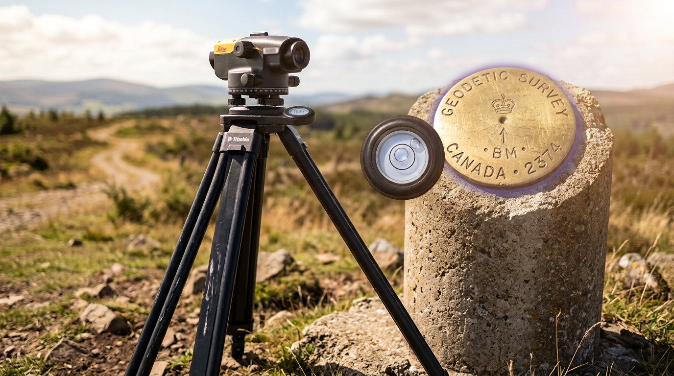
Figure 5. A clock's height above the geoid is a fact a surveyor already owns; the network only borrows it. — Image prompt and art direction by Brecht Corbeel; generation pending.

The Loop That Closes for the Wrong Reason

A tempting shortcut suggests itself immediately: pick any closed loop of clocks and sum the edge readings around it. If the sum fails to return to zero, something has broken the idea that a single scalar potential — curved or otherwise — assigns each clock one honest number. Formally, define the fitted residual

r := \left[I - B\left(B^\top C^{-1}B\right)^{+}B^\top C^{-1}\right] y,

the part of y that weighted least squares could not explain with any node potential at all. It is tempting to read a nonzero r as curvature declaring itself. That reading is wrong, and the reason is worth deriving rather than waving at.

Weighted least squares achieves zero residual on any data that lie exactly in the range of B. If y truly equals B\phi_{\rm true} for some vector \phi_{\rm true} — meaning a genuine, single-valued scalar potential sits at every node, however violently curved the spacetime that produced it — then \phi_{\rm true} itself drives the weighted sum of squares to exactly zero, which is the smallest value the nonnegative objective can take, so the fitted values equal y exactly and r \equiv 0. This holds independent of how strongly \phi varies from node to node, independent of C, and independent of the graph’s shape, because it is a fact about linear regression, not about gravity: any closed loop of static clocks, in any static spacetime whatsoever, closes exactly, because a sum of consecutive differences of a single-valued function around a closed path telescopes to zero by arithmetic alone. Curvature never has to intervene to make that true, and no amount of it can make that false.

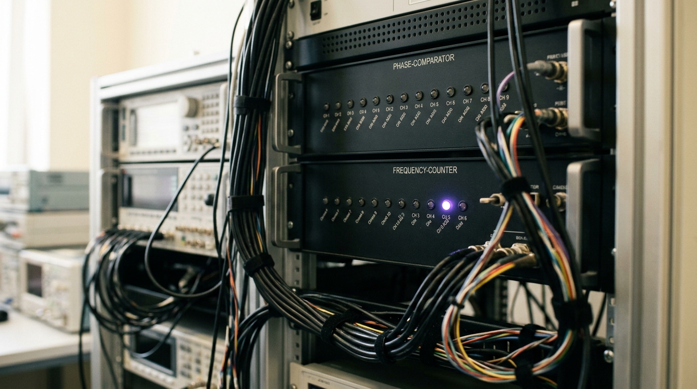
Figure 6. The rack reports a ratio between two clocks; whether that ratio closes around a loop is a question it cannot answer alone. — Image prompt and art direction by Brecht Corbeel; generation pending.

What r is actually sensitive to follows from the same argument in reverse. The null space of B has dimension equal to the number of connected components of the network graph; for a connected network it is exactly one-dimensional, spanned by the all-ones vector, because B\phi = 0 forces \phi_i = \phi_j across every edge and connectivity propagates that equality to every node. By rank–nullity, a connected tree — with exactly |V|-1 edges for |V| nodes — has an incidence matrix of full row rank, meaning that for any data whatsoever a \phi exists reproducing it exactly. A tree, in other words, cannot fail to close, on any data, ever; it carries zero redundant edges and therefore zero capacity to audit itself. Only once a network graph contains at least one independent cycle — one edge beyond a spanning tree — does y have anywhere to fall outside the range of B, and only then does a nonzero r become a genuine statement: that some edge or edges are not explained by any per-node scalar at all. What can produce that failure is a rotating platform’s asymmetric contribution to a link, an uncorrected fibre-length drift, a miscalibrated clock, or a bad connector — never curvature, because curvature is already fully compatible with a perfectly closing loop.

Figure 2. Every edge in the network is a claim that a photon kept its phase; the claim is checked here, not assumed. — Image prompt and art direction by Brecht Corbeel; generation pending.

What Actually Snaps the Loop Open

Real terrestrial clocks are not simply static; they corotate with Earth, and their genuinely single-valued potential is the geopotential W(\mathbf x) := \Phi_{\rm grav}(\mathbf x) - \tfrac12|\boldsymbol\Omega \times \mathbf r|^2, gravitational potential combined with the centrifugal term for Earth’s rotation rate \boldsymbol\Omega. Because W is a smooth, single-valued function of position in the corotating frame for any fixed \Omega, folding it into the node potential \phi := W/c^2 preserves exact loop closure for any network of clocks that are themselves at rest relative to the rotating Earth — precisely the convention already standard in relativistic geodesy [4, 3].

A loop opens, instead, whenever some edge’s own realization is not simply a difference of two corotating nodes’ W. The clearest documented case is the relativistic Sagnac effect: a synchronization or comparison signal that does not itself corotate with the network — a one-way satellite time transfer, or any path analyzed against a non-rotating inertial frame — picks up an explicit timing correction \Delta t_e = (2/c^2)\,\boldsymbol\Omega \cdot \mathbf A_e, where \mathbf A_e is the area swept by that specific link’s path, projected onto Earth’s equatorial plane. That expression carries units of time, while an edge datum is a dimensionless log frequency ratio, so what actually enters the edge is s_e = \Delta t_e/T for the averaging interval T over which the comparison is gated; this is exactly the term without which the Global Positioning System’s own time transfer disagrees with ground clocks by an amount well outside its design tolerance [10]. Whenever an edge’s own physical realization departs from plain node-to-node W-differencing in this way, the correct response is to model s_e explicitly on that edge — not to let it distort the fitted \hat\phi, and not to write it off as an unexplained curvature signal. The size of an uncorrected Sagnac term is worth putting a number to, because it is easy to underestimate. Take an illustrative closed network loop enclosing a continental-scale area of 2.5\times10^{11}\,\mathrm{m^2} — a square roughly five hundred kilometres on a side, comparable to the geographic span already reached by real international fibre links — at a latitude where the projected area onto Earth’s equatorial plane is close to the full value. With Earth’s sidereal rotation rate \Omega \approx 7.292\times10^{-5}\,\mathrm{rad\,s^{-1}} [10], the accumulated timing offset is \Delta t = 2\Omega A/c^2 \approx 2(7.292\times10^{-5})(2.5\times10^{11})/(8.988\times10^{16}) \approx 4.1\times10^{-10}\,\mathrm s, a little over four hundred picoseconds. Gated at the one-second averaging interval conventional for this comparison, the corresponding dimensionless edge bias is s = \Delta t/T \approx 4.1\times10^{-10} — eight to nine orders of magnitude larger than any clock’s own fractional instability. A loop of that size realized through any link geometry that does not automatically cancel this term — a one-way relay, most obviously — would swamp every other effect in this article before curvature or a fault ever entered the picture, which is exactly why the term has to be modelled on its own edge rather than left to contaminate the fitted node potentials. A real network built to search for exactly this kind of anomaly is the four-station European fibre link connecting clocks in France, Germany, the United Kingdom, and Italy, which compared measured frequency ratios against those predicted from independently known geopotential differences and searched for any residual daily variation tied to Earth’s motion, rather than to gravity [7]. A miniature, five-node laboratory array built expressly to test differential redshift at the one-centimetre scale shows the same logic operating at the opposite end of the size range: five atomic ensembles, four independent height differences, and a fractional frequency gradient measured and checked against the value gravity alone predicts [2]. In neither case does a nonzero comparison certify curvature; in both, it certifies — or fails to certify — that the network’s own bookkeeping accounted for everything that was not a per-node scalar.

An Elevator Can Fake the Slope, Never the Bend

The deeper question the loop-closure argument sets aside is what happens once loop closure has already been confirmed — once a single, well-behaved \hat\phi genuinely fits every edge. Does a nonzero slope in that fitted potential mean anything has curved? The equivalence principle’s oldest thought experiment already answers no, and the answer can be made exact rather than qualitative.

Consider a uniformly accelerated laboratory in otherwise empty, flat spacetime — Einstein’s elevator, given by the exact Rindler metric in coordinates comoving with an observer under constant proper acceleration g:

ds^2 = -U(Z)^2\,dx_0^2 + dZ^2 + dx^2 + dy^2, \qquad x_0 := ct, \qquad U(Z) := 1 + \frac{gZ}{c^2}.

This is an exact solution describing flat Minkowski spacetime in non-inertial coordinates, not a weak-field approximation. A clock held static at height Z has d\tau = U(Z)\,dt exactly, so two such clocks compare frequencies as \nu_2/\nu_1 = U(Z_1)/U(Z_2) to all orders — the same exact redshift formula an accelerating rocket produces for light climbing or falling inside it. The node potential is \phi(Z) = \ln U(Z) = \ln(1 + gZ/c^2), and its first derivative at Z=0 is \phi' = g/c^2: a nonzero, entirely real, measurable slope. A network of clocks bolted to this elevator’s walls would report exactly the nonzero edge data a network in a genuine gravitational field reports at the same order. If a nonzero slope alone were curvature, this elevator would be curved. It is not; by construction its spacetime is exactly flat, and the geodesic deviation between any two nearby free-falling test particles inside it is exactly zero at every instant, because flatness is a property of the manifold and does not care what coordinates — accelerated, rotating, or otherwise — a particular family of observers happens to use.

What must therefore vanish, identically, is not the slope but the correctly defined curvature-frame component built from it. For any static metric of the form ds^2 = -U(\mathbf x)^2\,dx_0^2 + \delta_{ij}\,dx^i dx^j — flat spatial slices, all the position dependence carried by U — the only nonzero Christoffel symbols are \Gamma^0_{0i} = \partial_i \ln U = \phi_{,i} and \Gamma^i_{00} = U^2\phi_{,i}, both following directly from the metric’s definition. Substituting into the Riemann tensor’s defining combination for the mixed component R^i{}_{0j0}, every term built from purely spatial Christoffels vanishes because the spatial slices are exactly flat, and the two surviving pieces are \partial_j\Gamma^i_{00} and -\Gamma^i_{0\lambda}\Gamma^\lambda_{j0}. Expanding \partial_j(U^2\phi_{,i}) = U^2\phi_{,i}\phi_{,j} + U^2\phi_{,ij} and \Gamma^i_{00}\Gamma^0_{j0} = U^2\phi_{,i}\phi_{,j}, the two copies of \phi_{,i}\phi_{,j} cancel exactly, leaving

R^i{}_{0j0} = U^2\left(\phi_{,ij} + \phi_{,i}\,\phi_{,j}\right).

The function U appearing throughout this construction is exactly what the initial-value formulation of general relativity calls the lapse: the local rate at which proper time elapses across a chosen family of spatial slices, the same static-spacetime object standard treatments of Killing symmetries already build on [14]. Nothing in the derivation above depends on that name; it is worth stating only because it confirms that U is not a quantity invented for this network — it is the same function relativists already use to slice a spacetime into space-plus-time, borrowed here rather than redefined.

Check it against the elevator directly: \phi = \ln(1+gZ/c^2) gives \phi' = (g/c^2)/U and \phi'' = -(g/c^2)^2/U^2 = -(\phi')^2 exactly, for every Z, not merely at leading order. The bracket \phi_{,ij}+\phi_{,i}\phi_{,j} vanishes identically, and so does R^i{}_{0j0} — confirming, by direct calculation rather than appeal to intuition, that a uniformly accelerated frame carries exactly zero curvature no matter how large its slope g becomes. The naive second difference of \ln U alone, without the quadratic correction, does not vanish in this case — a fact worth stating plainly, because it is exactly the trap a network audit could fall into if it used \phi_{,ij} by itself as its curvature signal.

The Component the Bend Leaves Behind

Define the network’s curvature-diagnosing observable directly from this result, restoring physical units through the relation between coordinate acceleration and proper time for a static observer,

\mathcal T_{ij} := c^2\left(\phi_{,ij} + \phi_{,i}\,\phi_{,j}\right),

a symmetric rank-two tensor in the local spatial frame of the static observers, with units of inverse time squared — the Eötvös units already standard in gravity-gradient surveying, where 1\,\mathrm E = 10^{-9}\,\mathrm{s^{-2}}. Under a rotation of the local spatial axes it transforms as an ordinary rank-two tensor; under a change of which node is used as the additive reference for \phi it is unchanged, because it depends only on derivatives of \phi, never its value; and up to the factor U^2 \approx 1 negligible at the one-part-in-10^9 level for any terrestrial network, it is c^2 times the frame component R^i{}_{0j0} of the Riemann tensor in the static observers’ own rest frame — a genuine curvature quantity, reported honestly as one stated-frame component rather than a coordinate-free scalar invariant, exactly the caveat this construction owes a reader.

Two known limits anchor it. First, the elevator: \mathcal T_{ij} \equiv 0 for any uniformly accelerated frame, proven directly above — the “uniform potential difference is not curvature” claim, derived rather than asserted. Second, weak-field gravity: expanding \phi \approx \Phi/c^2 for small \Phi/c^2, the quadratic term \phi_{,i}\phi_{,j} is second order in the already-small ratio \Phi/c^2 and negligible next to the first-order term \phi_{,ij} \approx \Phi_{,ij}/c^2, so \mathcal T_{ij} \to \Phi_{,ij}, exactly the ordinary Newtonian tidal tensor of tower and satellite geodesy [15, 14]. The first derivative alone, meanwhile, recovers the textbook gravitational redshift these networks were already built to measure: y \approx g\Delta h/c^2, first isolated in a laboratory tower by Pound and Rebka to about ten percent precision [11], later confirmed to about seventy parts per million by a hydrogen maser flown to ten thousand kilometres and compared against its own ground twin over a two-way microwave link that explicitly separated the rocket clock’s proper time from the ground station’s [12], and exploited today as a design target: modern optical clock stability is explicitly tied to centimetre-scale height resolution because g\,(0.01\,\mathrm m)/c^2 \approx 1.09\times10^{-18} [8]. None of this network machinery invents a new redshift law; every first-derivative number above is the one general relativity already predicts, recovered exactly where known theory says it must be, with the additive-reference-clock gauge freedom identified earlier standing in for any true observer at infinity that a bounded terrestrial network will never possess.

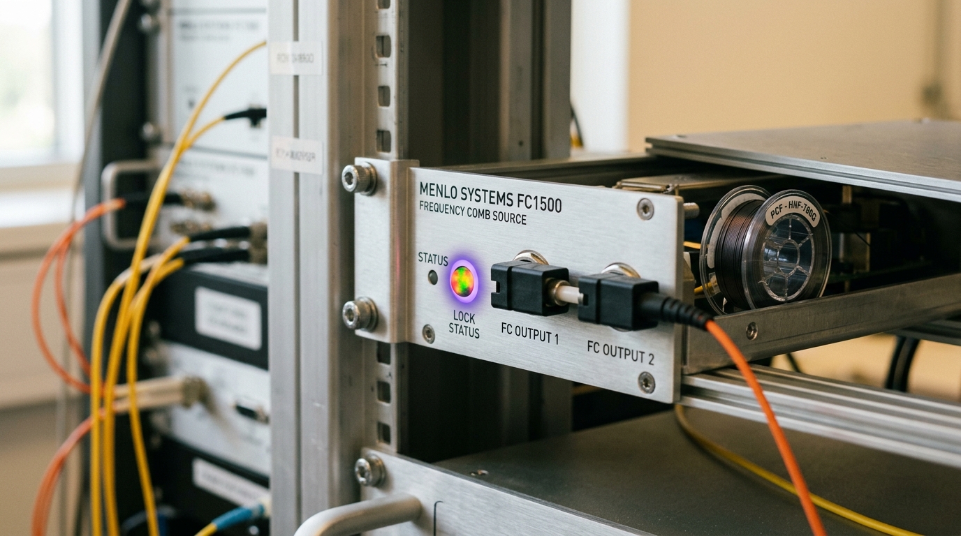
Figure 1. A comb converts an optical tick into a countable one; it never decides what the tick was measuring. — Image prompt and art direction by Brecht Corbeel; generation pending.

How Far Apart the Clocks Would Have to Stand

An exact analytic evaluation, not a simulation, fixes the scale this actually requires. Take three clocks stacked vertically at heights -h, 0, and +h near Earth’s surface, giving two edges y_1 = \phi(0)-\phi(-h) and y_2 = \phi(h)-\phi(0). Their difference is an exact finite-difference identity up to a Taylor remainder of order h^4:

y_2 - y_1 = \phi_{,zz}\,h^2 + O(h^4).

For Earth modelled as a point mass, \Phi(r) = -GM/r gives a radial second derivative of magnitude 2GM/R^3 and, since \Phi is harmonic in vacuum, transverse second derivatives of magnitude GM/R^3 with the opposite sign — a trace-free tensor in the exact ratio 2:{-1}:{-1}. With the standard gravitational parameter GM_\oplus = 3.986\times10^{14}\,\mathrm{m^3\,s^{-2}} and mean radius R_\oplus = 6.371\times10^{6}\,\mathrm m, this gives GM_\oplus/R_\oplus^3 \approx 1.541\times10^{-6}\,\mathrm{s^{-2}} and a radial magnitude of 3.08\times10^{-6}\,\mathrm{s^{-2}}, matching the standard geodetic free-air gravity gradient of about 3.086\times10^{-6}\,\mathrm{s^{-2}}, or 0.3086 milligal per metre, to three figures [15]. So \phi_{,zz} \approx 3.08\times10^{-6}/c^2 \approx 3.43\times10^{-23}\,\mathrm{m^{-2}}.

Take each edge’s fractional-frequency comparison uncertainty to be \sigma_y = 1\times10^{-18}, the stability optical clocks have already demonstrated is what centimetre-level geodesy requires [8]. The combined noise on the independent-edge difference y_2-y_1 is \sqrt2\,\sigma_y. Setting signal equal to noise, \phi_{,zz}\,h^2 = \sqrt2\,\sigma_y, gives

h = \sqrt{\frac{\sqrt2\,\sigma_y}{\phi_{,zz}}} = \sqrt{\frac{1.414\times10^{-18}}{3.43\times10^{-23}\,\mathrm{m^{-2}}}} \approx 203\,\mathrm m.

The fourth-derivative Taylor remainder at this height is smaller than the leading term by a factor of roughly 10^{-8}, confirming that the quadratic approximation used above is, for this purpose, exact. Two hundred metres of half-spacing — roughly four hundred metres end to end — is not a laboratory bench, but it is not exotic either: it is close to the height difference a transportable optical lattice clock actually used, linked to a second clock at the base of the Tokyo Skytree tower by fibre, to measure the ordinary first-derivative geopotential difference directly against independent levelling [9]. Comparable transportable-clock campaigns have carried a lattice clock into an underground laboratory and compared it against a distant reference over fibre [6], and connected two transportable clocks across a shorter urban baseline to test the redshift prediction itself against surveying [5]. None of those campaigns targeted the second-derivative signal computed here; the point of the calculation is that their baselines already sit at the right order of magnitude, not that any deployed network has yet reported this specific number.

It is worth being honest about how far current best precision still has to travel to make a genuinely compact version of this measurement realistic. The most precise fractional frequency resolution reported to date, 7.6\times10^{-21}, comes from comparing atoms at different heights inside a single shared optical lattice, where systematic effects common to both heights cancel almost completely [13]. If that exact resolution were ever achieved between two independently operated, physically separated network clocks — which is not what was demonstrated, and which faces a substantially harder common-mode-rejection problem — the same scaling gives h \propto \sqrt{\sigma_y} and a required half-spacing of roughly eighteen metres, a building’s height rather than a tower’s. That gap between a shared-trap demonstration and a genuinely remote one is exactly the kind of honest limitation this construction is required to state rather than paper over.

Figure 4. Moving the clock does not move the potential it will report; it only moves where the report is taken. — Image prompt and art direction by Brecht Corbeel; generation pending.

The Pattern a Spinning Platform Cannot Copy

Even a network that has cleared every check above owes one more: any fictitious, non-curvature contribution to a naive second difference has to be ruled out on its own terms, not merely assumed absent. A uniformly rotating platform’s centrifugal potential, -\tfrac12|\boldsymbol\Omega\times\mathbf r|^2, has a nonzero Hessian too — for rotation about the z-axis, \mathrm{diag}(-\Omega^2,-\Omega^2,0) — but that Hessian is exactly constant across any laboratory-scale network, tied to a rotation axis independently known from astrometry to extraordinary precision, and entirely absent from the trace-free, 2:{-1}:{-1}, 1/r^3-falling pattern a genuine point-like or spherical mass produces. A real curvature signal has to fall as the network’s baseline moves farther from the source, has to keep its stretching axis pointed at the local vertical as the network is relocated, and has to hold the exact 2:{-1}:{-1} eigenvalue ratio once any independently known rotational or accelerated-frame contribution has been subtracted using its own, separately measured parameters — never fitted freely alongside the curvature term, which would let the two masquerade as each other.

Earth’s own centrifugal contribution is the concrete case worth sizing, precisely because it is not negligible enough to ignore by assumption. With \Omega \approx 7.292\times10^{-5}\,\mathrm{rad\,s^{-1}} fixed by astrometry to far more figures than any clock network could hope to determine on its own [10], the centrifugal Hessian has magnitude \Omega^2 \approx 5.32\times10^{-9}\,\mathrm{s^{-2}} — smaller than the radial tidal magnitude computed above by a factor of nearly six hundred, but not so much smaller that a network aiming to certify the 2:{-1}:{-1} ratio to good precision can skip subtracting it. Left in, it would masquerade as roughly a fifth of one percent of the genuine tidal signal, concentrated entirely in the horizontal plane and constant across the whole network — exactly the flat, source-independent signature the falloff-and-orientation test above exists to catch, and exactly why \Omega has to be subtracted using its own independently known value rather than absorbed into whatever the least-squares fit finds convenient. A measured tensor that fails any one of those three tests — wrong falloff, wrong orientation relative to the vertical, or an eigenvalue ratio left over after subtraction that does not converge to 2:{-1}:{-1} — has not detected spacetime curvature, whatever its magnitude.

Figure 3. A relay along the fibre preserves the phase, not the potential; the two are not the same promise. — Image prompt and art direction by Brecht Corbeel; generation pending.

What the Network Still Owes a Surveyor

None of this replaces gravimetry, levelling, or satellite geodesy, and none of it was built to. The construction’s whole ambition is narrower: given a set of clocks and their pairwise frequency ratios, say exactly what can and cannot be concluded, and say it before the data arrive rather than after. A closed loop of static clocks will close regardless of curvature, so treat a nonzero cycle residual as a fault, rotation, or drift alarm — never a gravity detector — and localize it using the network’s own graph structure, adding an explicit term for any edge whose realization departs from ordinary node-to-node potential differencing [10, 7]. Treat a nonzero first-derivative slope as the redshift general relativity has predicted and confirmed since a hydrogen maser rode a rocket to ten thousand kilometres [12], recoverable today at the level real transportable clocks already work at [6, 5]. And treat a nonzero, correctly constructed second-derivative estimator — never the raw second difference alone, always the quadratic-corrected combination this article derived and checked against an exactly flat elevator — as the only one of the three that is honestly entitled to the word curvature, reportable only as a stated-frame Riemann component, at a baseline this article’s own arithmetic puts within reach of towers already built rather than towers yet to be imagined [9, 2].

The kill criterion follows directly from the derivation rather than being appended to it: if a network’s fitted tidal estimator fails to shrink as its baseline moves away from a known mass, fails to track the local vertical as the network is relocated, or survives a proper subtraction of every independently known rotational and accelerated-frame contribution without settling toward the trace-free 2:{-1}:{-1} pattern derived above, the claim that curvature has been diagnosed is false, regardless of how large the raw number looks on a screen. What survives that test is not a new theory of gravity, a new force, or a new invariant beyond what general relativity already supplies. It is a way of making sure a clock network is only ever credited with having measured what its own arithmetic can actually distinguish — a bend in spacetime — and never with what any elevator, resting or accelerating, could have produced for free.

Three separate clocks of meaning have run through this construction and none of them was ever allowed to stand in for another: a clock’s own proper time, ticking in a vacuum chamber that has never once referred to any other apparatus; a coordinate time the network agrees to compute in, a bookkeeping convention rather than a measured quantity; and the single reference node against which every reported number is necessarily a difference, standing in for the observer at infinity a bounded terrestrial network will never actually have. Every genuine advance this article records — a proof that loop closure is silent about curvature, an exact identity that a uniformly accelerating frame satisfies and a curved one does not, a numerical baseline within reach of towers already standing — depends on keeping that three-way distinction in view at every step, and dissolves the moment any one of the three is quietly mistaken for another.

Sources

1. Christian Lisdat et al.. A Clock Network for Geodesy and Fundamental Science. Nature Communications (2016). DOI: 10.1038/ncomms12443.
2. Xin Zheng, Jonathan Dolde, Matthew C. Cambria, Hong Ming Lim, and Shimon Kolkowitz. A Lab-Based Test of the Gravitational Redshift with a Miniature Clock Network. Nature Communications (2023). DOI: 10.1038/s41467-023-40629-8.
3. Tanja E. Mehlstäubler, Gesine Grosche, Christian Lisdat, Piet O. Schmidt, and Heiner Denker. Atomic Clocks for Geodesy. Reports on Progress in Physics (2018). DOI: 10.1088/1361-6633/aab409.
4. Arne Bjerhammar. On a Relativistic Geodesy. Bulletin Géodésique (1985). DOI: 10.1007/BF02520327.
5. Masao Takamoto et al.. Test of General Relativity by a Pair of Transportable Optical Lattice Clocks. Nature Photonics (2020). DOI: 10.1038/s41566-020-0619-8.
6. Jacopo Grotti et al.. Geodesy and Metrology with a Transportable Optical Clock. Nature Physics (2018). DOI: 10.1038/s41567-017-0042-3.
7. P. Delva et al.. Test of Special Relativity Using a Fiber Network of Optical Clocks. Physical Review Letters (2017). DOI: 10.1103/PhysRevLett.118.221102.
8. W. F. McGrew et al.. Atomic Clock Performance Enabling Geodesy Below the Centimetre Level. Nature (2018). DOI: 10.1038/s41586-018-0738-2.
9. Tetsushi Takano et al.. Geopotential Measurements with Synchronously Linked Optical Lattice Clocks. Nature Photonics (2016). DOI: 10.1038/nphoton.2016.159.
10. Neil Ashby. Relativity in the Global Positioning System. Living Reviews in Relativity (2003). DOI: 10.12942/lrr-2003-1.
11. R. V. Pound and G. A. Rebka. Apparent Weight of Photons. Physical Review Letters (1960). DOI: 10.1103/PhysRevLett.4.337.
12. R. F. C. Vessot et al.. Test of Relativistic Gravitation with a Space-Borne Hydrogen Maser. Physical Review Letters (1980). DOI: 10.1103/PhysRevLett.45.2081.
13. Tobias Bothwell et al.. Resolving the Gravitational Redshift Across a Millimetre-Scale Atomic Sample. Nature (2022). DOI: 10.1038/s41586-021-04349-7.
14. Robert M. Wald. General Relativity. University of Chicago Press (1984).
15. Bernhard Hofmann-Wellenhof and Helmut Moritz. Physical Geodesy. Springer Vienna (2006). DOI: 10.1007/978-3-211-33545-1.

Originally published at https://absolutedigitalpublishers.com/articles/a-clock-network-can-diagnose-curvature-without-inventing-gravity.