How Fast Can a Horizon Learn Which Path You Took?

A decoherence rate is not yet a learning rate. This research program turns horizon-state overlap into distinguishability, decision information, and an explicit time at which a which-path record becomes too late to erase.

Revolutionary Life 75, Series D, No. 2 — this article is the paper's summary; the full text (PDF): https://absolutedigitalpublishers.com/papers/revolutionary-life-75-d02-horizon-which-path.pdf

The horizon is not an eye. The operational question is when the two conditional field states become distinguishable enough to constitute a which-path receipt. — Image prompt and art direction by Brecht Corbeel; generation pending.

Abstract

Semiclassical field calculations show that a stationary charged or massive spatial superposition near a Killing horizon can entangle with soft field modes and lose visibility. That result is inherited. The proposed research contribution is an operational translation from conditional horizon-state overlap to three quantities that must not be conflated: the Holevo information ceiling, the information obtained by an optimal binary which-path decision, and the irreducible record remaining after the best admissible future attempt to restore coherence. For an exponential pure-state overlap, the first two clocks can be calculated exactly and disagree by a finite factor. A third receipt clock requires the finite-time purification problem. The program compares Schwarzschild, Kerr, Rindler, ordinary-matter, and near-extremal charged-black-hole rate models; includes screening and quantum spectral-gap regimes in which no finite recording time exists; and blocks any claim of a result until boundary-resolved field states, clock conventions, numerical artifacts, and external review are complete.

How Fast Can a Horizon Learn Which Path You Took?

A black hole is not watching the experiment. It has no eye at the horizon, no pointer needle behind it, and no moment of comprehension. Yet a horizon can receive two different quantum field states depending on which arm of a spatial superposition was occupied. If those states become distinguishable, the missing interference outside and the available which-path evidence are two descriptions of the same entanglement.

The difficult word in the title is therefore not horizon. It is learn.

A decay of fringe visibility tells us how much phase coherence an outside interferometer has lost. It does not, by itself, tell us how many bits a particular measurement can extract, whether the relevant field state is pure, which region contains the evidence, or whether clever future control can still cancel part of the record. Calling every exponential a learning curve smuggles four questions into one symbol.

This article registers a calculation designed to separate them. It does not report a new black-hole result. The inherited field theory is already striking: a charged or massive body held in a stationary spatial superposition outside a black hole can entangle with soft field modes crossing the horizon, even when the opening and closing motions are made adiabatic enough to suppress ordinary radiation to infinity [1]. The result was generalized from black-hole event horizons to Killing horizons, including Rindler and de Sitter cases [2]. Rotating-horizon calculations then fixed coefficients in electromagnetic and scalar analogues and exposed an extremal screening limit [3].

What is proposed here is narrower: feed a verified conditional-state overlap into an explicit information ledger. The ledger has a visibility clock, a Holevo-ceiling clock, an optimal-decision clock, and an irrevocable-receipt clock. It returns infinity, not a dramatic finite number, whenever the physical rate vanishes. It keeps Killing time, proper time, and affine horizon parameters in separate columns. And it treats the phrase “the horizon learned” as shorthand for a state-discrimination task, never as consciousness or wavefunction collapse.

The headline question then becomes precise enough to have an embarrassing answer: sometimes the horizon can discriminate a path before it holds an irrevocable receipt; sometimes an ordinary warm conductor could keep a similar clock; and in some near-extremal quantum regimes the clock does not tick at all.

The mail slot is not an observer

Begin with an equal superposition of two localized alternatives,

|\Psi(0)\rangle= \frac{|0\rangle+|1\rangle}{\sqrt 2}\otimes|h_{\rm in}\rangle .

The labels zero and one denote paths, not energy eigenstates. After the system’s long-range field interacts with the inaccessible degrees of freedom, an idealized final pure state has the form

|\Psi(T)\rangle= \frac{|0\rangle|h_0(T)\rangle+ |1\rangle|h_1(T)\rangle}{\sqrt 2}.

Tracing out the field multiplies the off-diagonal element of the path density matrix by the conditional-state overlap

\nu(T)=\langle h_0(T)|h_1(T)\rangle, \qquad V(T)=|\nu(T)|.

Under balanced arms and otherwise ideal readout, V is the remaining fringe visibility. That statement belongs to ordinary complementarity, not black-hole mysticism. Englert derived a quantitative visibility–which-way bound for a two-path interferometer, and atom-interferometer experiments later measured visibility and distinguishability independently in agreement with the relation [11, 12].

The horizon papers supply a curved-spacetime mechanism for changing \nu. Danielson, Satishchandran, and Wald describe the conditional long-range fields as sourcing distinct coherent states of the radiation. Radiation reaching the horizon is a genuine independent degree of freedom rather than a merely constrained Coulomb field, so slow recombination cannot necessarily restore its overlap [1]. Their later causality argument has an instructive ancestor: if an interior observer could in principle distinguish the long-range fields of two exterior branches, consistency prevents that optional later measurement from deciding whether Alice’s already spacelike-separated interference survives. Quantized radiation and vacuum fluctuations jointly remove the paradox [10].

None of this says a horizon performs a laboratory measurement. The useful statement is conditional: branch zero prepares one state on a declared field algebra or region; branch one prepares another; the two states admit some distinguishability. “Record” names that correlation. “Learn” names the performance of an allowed decoding measurement. The reader must always be named.

Figure 1. Visibility loss, state distinguishability, and bits recovered by a decision rule are related, but they are not the same quantity. — Image prompt and art direction by Brecht Corbeel; generation pending.

This also separates the present problem from a different one with a similar title. Arrasmith, Albrecht, and Zurek studied a black hole itself in a spatial superposition and the Hawking radiation that reveals the hole’s position [16]. Here the black hole is the environment and the exterior charged or massive object is superposed. Swapping those roles changes the conditional states and the physical rate.

One overlap contains at least three inequivalent amounts of information

Assume for the moment that |h_0\rangle and |h_1\rangle are pure, normalized, and prepared with equal prior probability. Define their trace distinguishability

D(T)=\frac12 \left\| |h_0\rangle\langle h_0|- |h_1\rangle\langle h_1| \right\|_1.

For two pure states,

D(T)=\sqrt{1-V(T)^2}, \qquad V(T)^2+D(T)^2=1.

This is the first translation. A visibility of 0.6 corresponds to a trace distinguishability of 0.8; neither number is a bit count.

Helstrom’s binary decision theory supplies the minimum average probability of guessing the wrong path:

p_{\rm e}(T)=\frac{1-D(T)}{2} =\frac{1-\sqrt{1-V(T)^2}}{2}.

For the balanced pure-state problem, the minimum-error measurement induces a symmetric binary channel. Its recovered decision information is

I_{\rm dec}(T)=1-h_2[p_{\rm e}(T)],

where

h_2(p)=-p\log_2p-(1-p)\log_2(1-p)

is binary entropy. The first equation inherits quantum minimum-error detection [14]. The second is ordinary mutual information for the resulting binary channel. It answers a concrete question: if one path bit was chosen fairly and one optimized single-shot yes/no measurement was made, how many bits did that decision convey on average?

There is another number in the same pair of states. The Holevo quantity of the equal-prior pure ensemble is

\chi_H(T)= h_2\!\left(\frac{1+V(T)}{2}\right).

It is the von Neumann entropy of the average conditional state because each conditional state is pure. Holevo’s theorem makes this quantity an upper bound on classical information accessible through a quantum measurement, not a guarantee that an arbitrary one-copy receiver attains it [13]. Fuchs and Caves developed ensemble-dependent bounds that make the gap between a state’s information content and a receiver’s accessible information explicit [15].

That gap is not semantic. At V=0.5, the Holevo ceiling is about 0.811 bits. The minimum-error binary decision yields about 0.646 bits. A sentence saying “the horizon contains 0.811 bits, therefore Bob can read 0.811 bits” has silently replaced an upper bound with a decoder.

For mixed conditional states, unequal path priors, restricted measurements, or an accessible subregion rather than the full horizon field, the pure-state equalities above do not survive unchanged. Trace distance remains an operational decision quantity, and the Holevo quantity can still be computed for a declared ensemble, but overlap alone no longer determines everything. The proposed pipeline must receive density operators or a justified pure coherent-state reduction; it cannot infer missing state structure from a fitted contrast curve.

An exponential has more than one recording time

Suppose a field calculation actually justifies

V(T)=e^{-\Gamma T},

where \Gamma has units of inverse time in the explicitly named time coordinate. Define a confidence deficit \delta. A Holevo-ceiling time is

T_\chi(\delta)= \inf\{T:\chi_H(T)\geq1-\delta\},

and a minimum-error decision time is

T_{\rm dec}(\delta)= \inf\{T:I_{\rm dec}(T)\geq1-\delta\}.

Both are deterministic transformations of the assumed overlap law. Neither is a new field-theory result. Numerically inverting the two binary-entropy equations gives:

• Allowed information deficit \delta — overlap at Holevo threshold — \Gamma T_\chi — overlap at decision threshold — \Gamma T_{\rm dec}
• 0.1 — 0.367961 — 0.999777 — 0.226435 — 1.485297
• 0.01 — 0.117605 — 2.140426 — 0.058633 — 2.836452
• 0.001 — 0.037229 — 3.290676 — 0.016143 — 4.126270

The table is an analytic computation performed for this proposal, not a simulation or an observation. It says that a common phrase such as “one decoherence time” is underspecified. At the 0.9-bit threshold, a Holevo ceiling appears at almost exactly one inverse rate, while the specified decision task needs about 1.49 inverse rates. At the 0.999-bit threshold the two clocks read about 3.29 and 4.13. The disagreement is finite and predictable.

No threshold in that table is a constant of nature. The choices of equal path priors, one binary use, a bit-valued score, and a tolerated deficit all belong to the question an observer asks. A rare-path experiment, a repeated decoder, or a loss function that prices false positives more heavily would produce a different clock from the same conditional states. The honest output is therefore the complete information-versus-time curve together with several declared operating points, not a single crossing selected because it resembles an expected decoherence time. This sensitivity is useful: if two proposed horizon mechanisms have similar visibility decay but rank differently under a physically motivated asymmetric decision cost, the operational translation has revealed a distinction. If every sensible score merely rescales the same curve, the extra clocks have added presentation rather than physics.

Figure 2. One exponential produces different threshold times for a Holevo ceiling, an optimal binary decision, and an irrevocable record. — Image prompt and art direction by Brecht Corbeel; generation pending.

This gives the research program its first hard rule: no plot may label an axis “information recorded” unless its legend says which information, which receiver, which prior, and which measurement restrictions. Visibility, Holevo information, and decision information may share a horizontal axis. They may not share a name.

There is also a useful limit. If \Gamma=0, then V=1, D=0, and both threshold times are infinite for every \delta<1. A code path that divides by zero, clips the answer to its plotting horizon, or prints a spectacularly large finite number has converted a physical no-record regime into graphics.

The rate comes from field theory, not from the information ledger

Gralla and Wei calculate the large-holding-time overlap for nonextremal bifurcate Killing horizons in electromagnetic and Klein–Gordon analogues. In their natural-unit convention,

V(T)=\exp\!\left(-\frac{C\kappa T}{2}\right),

so the adapter into the exponential ledger is

\Gamma=\frac{C\kappa}{2}.

Here C is their dimensionless decohering flux, \kappa is surface gravity with inverse-time units in the chosen normalization, and T is the associated Killing time. Their calculation fixes the numerical factor absent from earlier scaling estimates and evaluates C for an observer on the symmetry axis of a Kerr black hole [3]. The information equations above neither alter C nor derive \kappa. They translate a verified overlap into operational thresholds.

Clock discipline matters near a horizon. A static laboratory’s proper time and the asymptotic Killing time differ by the lapse. Affine parameters on the horizon enter the mode decomposition differently again. The product \Gamma T must be dimensionless after the rate and duration have been expressed in the same convention. The planned code carries a clock identifier with every rate object and refuses to multiply mismatched clocks. Relabeling an asymptotic rate as a local proper-time rate can create an apparent redshift enhancement or suppression without changing the physics.

Danielson, Satishchandran, and Wald’s broader Killing-horizon analysis shows why the rate is not simply ordinary radiation power. From the Rindler description, soft photons or gravitons cross the horizon with negligible boost energy while the expected number of entangling quanta grows with holding time. From an inertial description, the same process can be represented through radiation reaching null infinity [2]. Which description is convenient depends on the observer and boundary, but Alice’s final coherence cannot depend on a verbal choice between them.

Recent work has made the local account sharper. Wilson-Gerow, Dugad, and Chen map the effect to random forces in a worldline-localized open-system description and connect steady decoherence to Ohmic friction plus finite-temperature fluctuations [4]. Danielson, Satishchandran, and Wald calculate the same Schwarzschild effect from local two-point functions in Alice’s laboratory and distinguish Unruh, Hartle–Hawking, and Boulware state choices; their published paper also carries an August 2025 correction to signs in two equations, a reminder that a rate importer must record version and state convention [6].

Figure 5. A global horizon account and a local fluctuation account can describe the same loss of coherence; double-counting them would manufacture a rate. — Image prompt and art direction by Brecht Corbeel; generation pending.

Global horizon flux and local field fluctuations are not two decoherence channels to be added. They are alternative accounts of the same correlations in the regimes where the derivations agree. The numerical ledger therefore has a provenance graph. Rates tagged global-horizon and local-correlator may be compared. They may not be summed unless a derivation establishes statistically independent physical environments.

The same restraint applies to ordinary matter. Biggs and Maldacena formulate the problem using fluctuating multipole operators and show that finite-temperature ordinary systems can produce qualitatively similar decoherence; in the electromagnetic comparison, ordinary conducting matter can even be quantitatively comparable under matched conditions [5]. A successful horizon-information clock would not establish that only horizons can learn. It would establish how to translate a particular environment’s conditional-state dynamics into a declared inference task.

A receipt can remain partly returnable after the envelope is closed

The exponential calculation assumes that T labels a completed preparation–hold–recombination protocol. It does not answer how much information has become irrevocable at an intermediate cutoff t_c. That distinction became unavoidable when Danielson, Kudler-Flam, Satishchandran, and Wald solved a finite-time optimization problem: given the entangling radiation already past a horizon cross-section, what future field purification best preserves Alice’s coherence? Their optimal future can be nonintuitive. Even after Alice has brought the branches together, reopening and manipulating the superposition can sometimes reduce the final decoherence [7].

So a horizon crossing is not automatically a stamped receipt for a classical path bit. The quantum field vacuum is entangled across time and region. A partial record at a cutoff can be completed by different future purifications, and the one maximizing final branch overlap need not correspond to “stop moving everything now.”

Define \mathcal A(t_c) as a preregistered set of physically admissible future protocols after the cutoff. It must specify which controls Alice retains, their duration, energy, acceleration, localization, and boundary conditions. For each u\in\mathcal A(t_c), let \rho^{u}_{0,H} and \rho^{u}_{1,H} be the completed conditional states on the declared horizon algebra. Then define an irreducible distinguishability envelope

D_{\rm irr}(t_c)= \inf_{u\in\mathcal A(t_c)} \frac12\left\|\rho^{u}_{0,H}-\rho^{u}_{1,H}\right\|_1.

The infimum asks how little path distinguishability remains after the best allowed attempt to erase it. For equal priors, an associated unavoidable decision information is

I_{\rm irr}(t_c)= 1-h_2\!\left(\frac{1-D_{\rm irr}(t_c)}{2}\right).

Finally, the proposed horizon receipt time is

T_{\rm receipt}(\delta)= \inf\{t_c:I_{\rm irr}(t_c)\geq1-\delta\}.

These are proposed definitions, not results from the 2025 optimization paper. They deliberately make admissible control part of the quantity. If \mathcal A grants arbitrary global unitaries on the horizon, the record can become fictitiously erasable. If it permits only “do nothing,” receipt time collapses into an ordinary decay threshold. A physically useful answer must live between those caricatures.

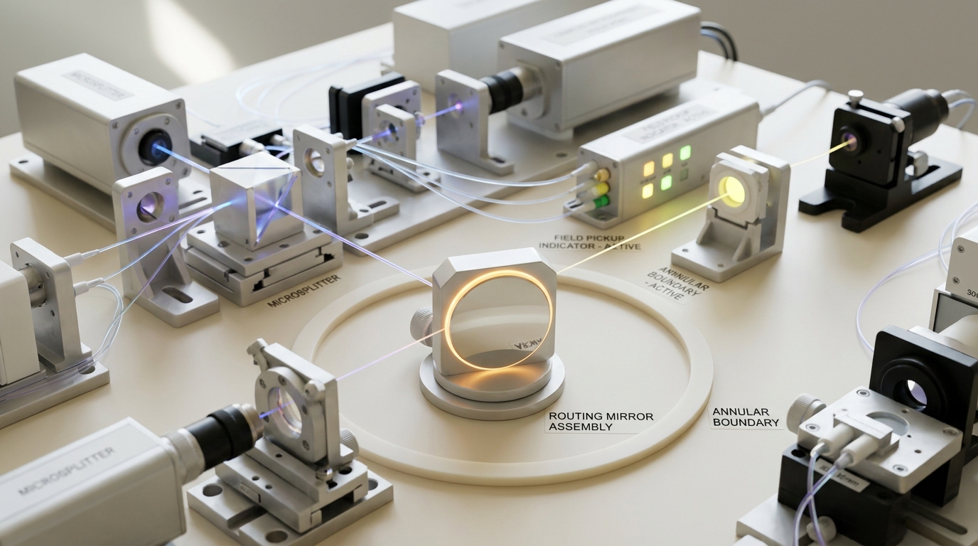
Figure 3. At a finite cutoff, closing the paths need not maximize restored coherence; the best future protocol may reopen and reshape the soft field. — Image prompt and art direction by Brecht Corbeel; generation pending.

The receipt clock could be later than the decision clock calculated from the final state of one fixed protocol. That would mean a decoder could already extract substantial which-path information from the current conditional states, yet Alice still retains a future maneuver that makes the completed states less distinguishable. “Readable now” and “no longer returnable” are different properties of a quantum record.

The program will not assume D_{\rm irr}(t_c) is monotone. Monotonicity may follow only when the admissible-control set shrinks consistently with time and the horizon subalgebras are nested in the required sense. If reopening grants a qualitatively new route at a later cutoff, a naïve implementation could violate the ordering. The paper must prove the conditions or report the nonmonotonicity as a definition failure.

Some horizons have a recording dead zone

The nonextremal exponential is not universal. Gralla and Wei find that at zero surface gravity a scalar/Klein–Gordon analogue can cross to power-law overlap,

V(T)=\left(\frac{T}{T_0}\right)^{-C},

while in their electromagnetic extremal Kerr limit the relevant horizon flux is expelled: both the surface gravity and electromagnetic decohering flux vanish because the external field does not penetrate the horizon [3]. For a genuine power law with C>0, a threshold clock scales as a power of the required overlap rather than a logarithm. For the screened electromagnetic case, no horizon record accumulates through that channel.

The sharper 2026 challenge comes from quantum rather than semiclassical extremality. Biggs and Trezzi study near-extremal charged Reissner–Nordström black holes with quantum fluctuations of the near-horizon geometry. In their electromagnetic single-charge-superposition setup, a spin-induced gap in the black-hole spectrum makes the late-time decoherence rate vanish when the energy above extremality lies below

E_b=\frac{G_N}{r_0^3} =\frac{\pi}{r_0S_0}

in their natural-unit conventions. They establish the zero through quartic order in the interaction and conjecture it to all orders for the stated opposite-dipole geometry; above the gap, the quantum-corrected rate remains below the semiclassical prediction [8]. The work is a 2026 preprint, not a settled experimental fact, and its zero does not automatically extend to arbitrary charge configurations or to the gravitational channel.

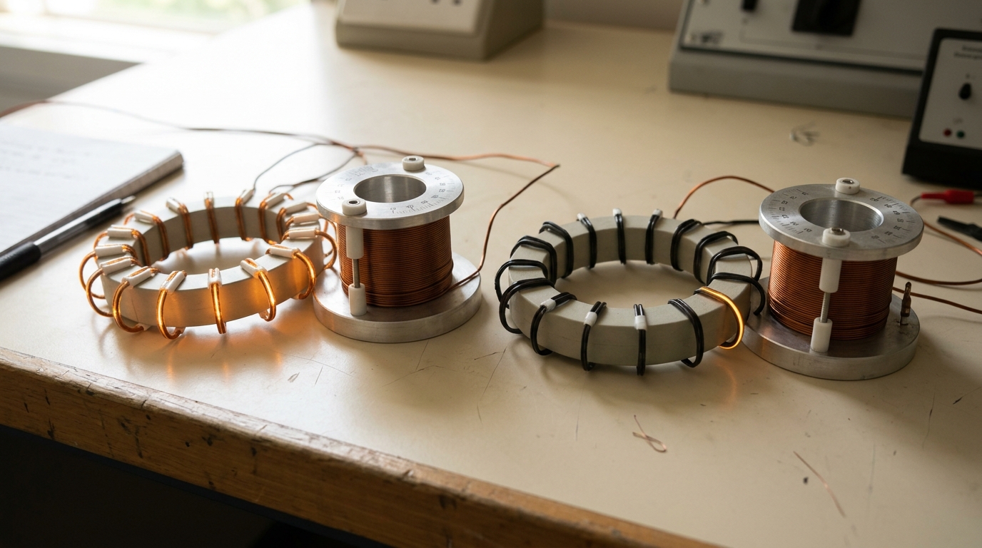
Figure 4. A horizon clock can stop: classical flux expulsion and quantum spectral gaps create regimes in which the assumed exponential rate vanishes. — Image prompt and art direction by Brecht Corbeel; generation pending.

This is exactly why the rate adapter needs a domain mask. For every point in mass, charge, spin, source geometry, distance, field type, vacuum state, and holding-time parameter space, the pipeline records one of four statuses:

1. rate derived and positive;
2. rate derived and zero;
3. approximation invalid;
4. rate not yet calculated.

Status four must never be plotted as zero. Status two must never be replaced by a tiny positive floor for convenience. A color map that confuses them turns theoretical ignorance and physical screening into the same shade.

Another 2026 preprint provides a useful but bounded robustness check. Batista, Landulfo, Mann, and Matsas give a nonperturbative Unruh–DeWitt-detector treatment of the DSW mechanism for a gapless detector on uniformly accelerated superposed trajectories coupled to a massive scalar field [9]. It supports controlled analysis beyond a lowest-order expansion in that model. It is not an electromagnetic Kerr calculation, not a graviton calculation, and not permission to transfer its conclusions across the dead-zone boundary.

The horizon clock must therefore be modular. A semiclassical Schwarzschild rate, a Kerr electromagnetic rate, a Rindler detector model, and a quantum-corrected near-extremal charged rate are different providers. The information layer can compare their consequences because it consumes conditional states or overlap laws with units and domains. It cannot make them one theory by placing their curves on the same axes.

The unrun calculation is a map with receipts, not a heroic number

The first numerical artifact will be a versioned rate-to-record notebook and command-line program. It will not solve quantum gravity. Its job is to expose every assumption between an imported field calculation and a sentence about learned information.

For each provider, the configuration records:

• the spacetime and horizon type;
• black-hole mass, angular momentum, charge, and extremality measure;
• source charge or mass, branch separation, orientation, distance, opening time, holding time, and closing time;
• electromagnetic, scalar, or linearized-gravity channel;
• field state and boundary decomposition;
• the coordinate in which the rate is defined and its conversion to the laboratory clock;
• whether conditional states are pure, mixed, or represented only by a justified asymptotic overlap;
• the validity inequalities and their numerical margins;
• the paper version, equation identifier, unit convention, and any known correction.

The program first reproduces published overlap or decoherence curves inside their stated regimes. Only then does it calculate D, p_{\rm e}, \chi_H, I_{\rm dec}, and threshold times. A separate finite-time module approximates the admissible-future optimization needed for D_{\rm irr}. Its result is labeled exploratory until it reproduces benchmark purification cases from the 2025 work.

The boundary ledger is as important as the state calculation. The completed radiation may have contributions on the horizon and at null infinity. If the article asks what the horizon knows, it must trace or restrict to the horizon subsystem rather than infer horizon information from Alice’s total visibility loss. A photon at null infinity can destroy Alice’s interference without placing a readable record behind the horizon. Conversely, a conditional horizon state can be difficult for any localized interior observer to collect even when its global trace distance is large.

That motivates two access models. The global algebra score permits the optimal measurement on the entire declared horizon state. The causal collector score restricts the measurement to the world tube and duration of a modeled interior receiver. Their difference is an access gap,

\Delta I_{\rm access}(T)= I_{\rm global}(T)-I_{\rm collector}(T).

This gap is another proposed observable. It prevents the phrase “information is in the horizon state” from becoming “one observer can gather it.” The global score is a capacity statement; the collector score is an engineering task constrained by causal geometry.

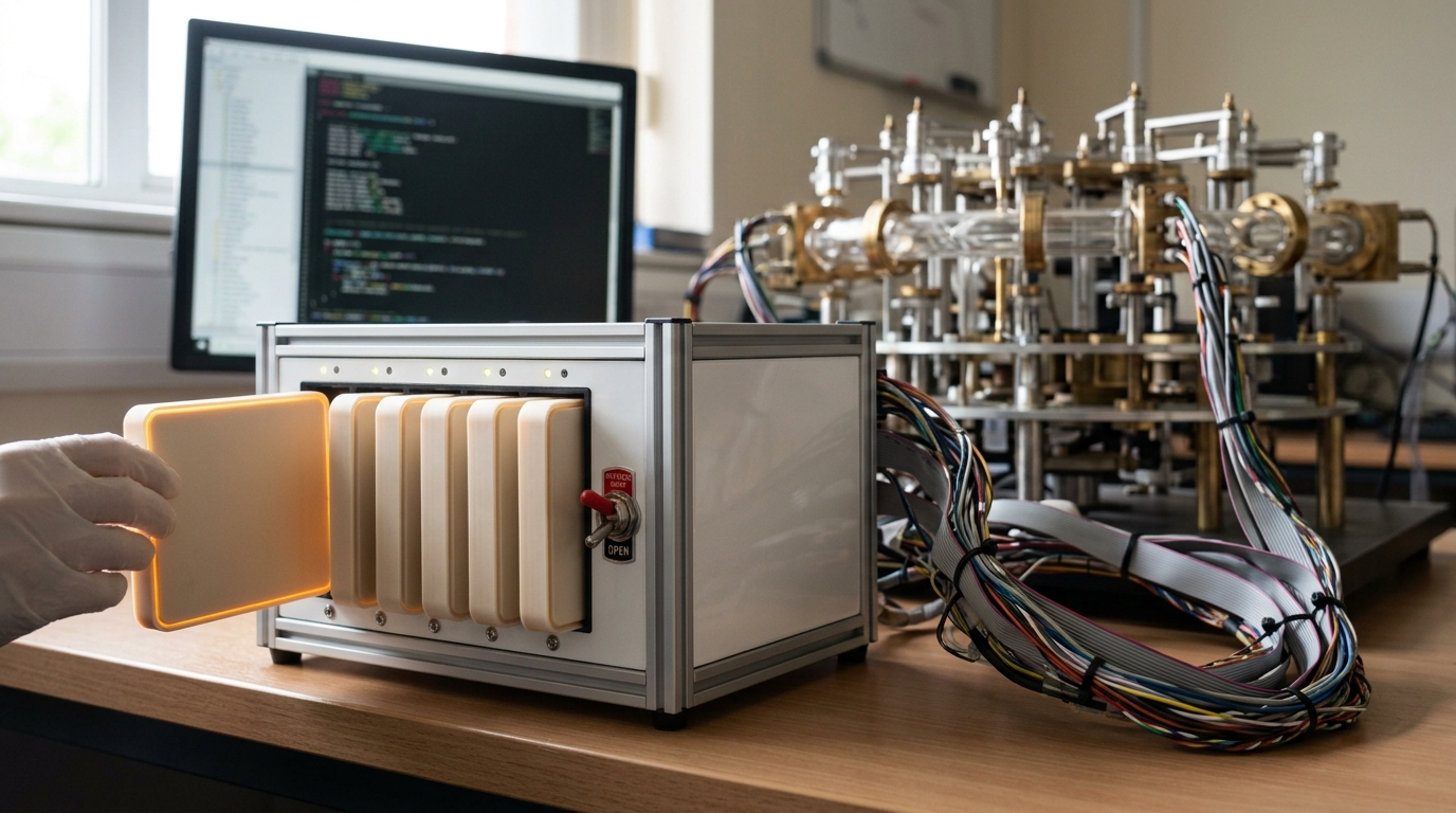
Figure 6. The information translation is analytic; the spacetime map remains an unrun program until its field states, boundaries, clocks, and controls are fixed. — Image prompt and art direction by Brecht Corbeel; generation pending.

No numerical spacetime map, collector optimization, or receipt curve has been run for this article. The only calculated values reported here are the dimensionless binary-entropy threshold inversions in the table, which follow from the explicitly assumed pure-state exponential. The companion paper must remain visibly incomplete until it contains the field-provider tests, saved configurations, raw outputs, environment lockfile, and independent subject-matter review.

Six ways the title can be wrong

The research program is designed to lose cleanly.

The field-state failure. A full boundary-resolved calculation could show that the horizon conditional states remain identical in a regime where a reduced phenomenological model assigned a positive \Gamma. Then there is no horizon which-path record, and the finite recording time is an artifact.

The provenance failure. Alice’s visibility may decay because of local apparatus noise, radiation to null infinity, or acceleration/control fields. If those contributions cannot be separated from the horizon channel, the calculation cannot answer the title even if it predicts total decoherence accurately.

The decoder failure. A large Holevo quantity on the global state may require a collective measurement unavailable to the modeled observer. If every causal collector remains near chance, saying that a horizon observer “learned” the path overstates a capacity bound. The access gap, not the global ceiling, becomes the result.

The receipt failure. If the value of T_{\rm receipt} changes without convergence as the admissible future-control family is enlarged, the new clock is not robust. It should be reported as protocol-relative or abandoned, not promoted as a property of the horizon.

The extremal failure. If screening, a spectral gap, or another selection rule makes the relevant rate vanish, no finite amount of holding time produces the proposed record through that channel. A null region is a physical prediction to preserve, not an inconvenience to smooth away.

The novelty failure. The rate-to-information translation may add no scientific discrimination beyond plotting V(T). If Holevo, decision, collector, and receipt thresholds never change a parameter ranking, regime boundary, or proposed test, then the new vocabulary is bookkeeping. The paper should reduce itself to a methods note or be withdrawn.

The strongest countermodel is mundane: the horizon is one thermal, dissipative quantum system among others. Warm-horizon and ordinary-matter analyses already make this countermodel quantitatively serious [4, 5]. The proposed framework accepts the demotion. Its goal is not to prove black holes uniquely observe. It is to price exactly what any conditional environment state allows a specified reader to infer.

The second countermodel is local: no global horizon account is needed in Alice’s laboratory. The local two-point-function formulation can reproduce the decoherence while making the operative noise visible in the lab [6]. That does not erase the horizon description; it forbids treating the two perspectives as independent evidence.

The third is temporal: “already crossed” does not equal “already irreversible.” The optimal-purification result makes that objection concrete [7]. Receipt time survives only if it incorporates the best physically allowed future, rather than declaring every partial trace permanent by notation.

What would count as a result

A successful first paper would not announce that black holes think. It would deliver five smaller things:

1. a reproduced conditional-overlap calculation with its regime and clock convention intact;
2. a checked translation into Holevo ceiling, minimum-error decision information, and threshold times;
3. a finite-time irreducibility envelope benchmarked against known optimal-purification cases;
4. a boundary-resolved comparison between global capacity and a causal collector;
5. a parameter map that displays positive-rate, zero-rate, invalid, and unknown regions separately.

The decisive comparison is not Schwarzschild versus Kerr for drama. It is fixed final visibility versus different operational questions. If two systems have the same V but different state mixedness, access geometry, or future controllability, the proposed ledger should give different answers. If it cannot, overlap already contains all the useful content and the extra machinery has failed its reason for existing.

The comparison also needs a negative control with no horizon. The same opening, holding, and closing trajectory should be evaluated beside an ordinary dissipative body and in the corresponding horizonless field state, with temperature and low-frequency response matched as closely as the models allow. This is not an attempt to subtract “ordinary” physics until something exotic remains. It asks whether the proposed clocks respond to conditional-state structure rather than to the word black hole. If matched environments give matched states, the ledger must give matched times. If it does not, the bug is in the translation.

There is a final conceptual limit. Decoherence is not collapse. A reduced path state can lose interference because phase information resides in correlations with a field. Nothing in the calculation selects a metaphysical interpretation of quantum mechanics. The horizon receipt records what a specified measurement can distinguish and what specified controls can no longer erase. It does not certify that one path became ontologically real.

That restraint makes the question better, not smaller. A horizon can be treated as a one-way boundary without being personified. A which-path field can become distinguishable without becoming public to every observer. A rate can become an information clock without becoming a universal clock. And an apparent receipt can remain partly returnable after the envelope has been closed.

The proposed result is therefore a refusal to let one exponential do four jobs. When the field theory gives a positive rate, the ledger asks which bit, for which reader, by which deadline, under which remaining control. When the rate vanishes, it prints infinity. That is how a horizon’s “learning” becomes a physical question rather than a metaphor with an equation beside it.

Sources

1. Daine L. Danielson, Gautam Satishchandran, and Robert M. Wald. Black Holes Decohere Quantum Superpositions. International Journal of Modern Physics D (2022). DOI: 10.1142/S0218271822410036.
2. Daine L. Danielson, Gautam Satishchandran, and Robert M. Wald. Killing Horizons Decohere Quantum Superpositions. Physical Review D (2023). DOI: 10.1103/PhysRevD.108.025007.
3. Samuel E. Gralla and Hongji Wei. Decoherence from Horizons: General Formulation and Rotating Black Holes. Physical Review D (2024). DOI: 10.1103/PhysRevD.109.065031.
4. Jordan Wilson-Gerow, Annika Dugad, and Yanbei Chen. Decoherence by Warm Horizons. Physical Review D (2024). DOI: 10.1103/PhysRevD.110.045002.
5. Anna Biggs and Juan Maldacena. Comparing the Decoherence Effects Due to Black Holes versus Ordinary Matter. arXiv (2024).
6. Daine L. Danielson, Gautam Satishchandran, and Robert M. Wald. Local Description of Decoherence of Quantum Superpositions by Black Holes and Other Bodies. Physical Review D (2025). DOI: 10.1103/PhysRevD.111.025014.
7. Daine L. Danielson, Jonah Kudler-Flam, Gautam Satishchandran, and Robert M. Wald. How to Minimize the Decoherence Caused by Black Holes. Physical Review D (2025). DOI: 10.1103/67vv-km43.
8. Anna Biggs and Stefano Trezzi. Not All Black Holes Decohere Quantum Superpositions. arXiv (2026).
9. Levy B. N. Batista, André G. S. Landulfo, Robert B. Mann, and George E. A. Matsas. Nonperturbative Danielson-Satishchandran-Wald Decoherence with Unruh-DeWitt Detectors. arXiv (2026).
10. Alessio Belenchia, Robert M. Wald, Flaminia Giacomini, Esteban Castro-Ruiz, Časlav Brukner, and Markus Aspelmeyer. Quantum Superposition of Massive Objects and the Quantization of Gravity. Physical Review D (2018). DOI: 10.1103/PhysRevD.98.126009.
11. Berthold-Georg Englert. Fringe Visibility and Which-Way Information: An Inequality. Physical Review Letters (1996). DOI: 10.1103/PhysRevLett.77.2154.
12. S. Dürr, T. Nonn, and G. Rempe. Fringe Visibility and Which-Way Information in an Atom Interferometer. Physical Review Letters (1998). DOI: 10.1103/PhysRevLett.81.5705.
13. Alexander S. Holevo. Bounds for the Quantity of Information Transmitted by a Quantum Communication Channel. Problems of Information Transmission (1973).
14. Carl W. Helstrom. Quantum Detection and Estimation Theory. Journal of Statistical Physics (1969). DOI: 10.1007/BF01007479.
15. Christopher A. Fuchs and Carlton M. Caves. Ensemble-Dependent Bounds for Accessible Information in Quantum Mechanics. Physical Review Letters (1994). DOI: 10.1103/PhysRevLett.73.3047.
16. Andrew Arrasmith, Andreas Albrecht, and Wojciech H. Zurek. Decoherence of Black Hole Superpositions by Hawking Radiation. Nature Communications (2019). DOI: 10.1038/s41467-019-08426-4.

Originally published at https://absolutedigitalpublishers.com/articles/how-fast-can-a-horizon-learn-which-path-you-took.