How AI Datacenter Interconnects Actually Work

Scale-up fabrics move data at the speed of a shared memory space; scale-out fabrics move it at the speed of a switch queue. A training job lives across both, and where the boundary falls decides how fast the cluster actually trains.

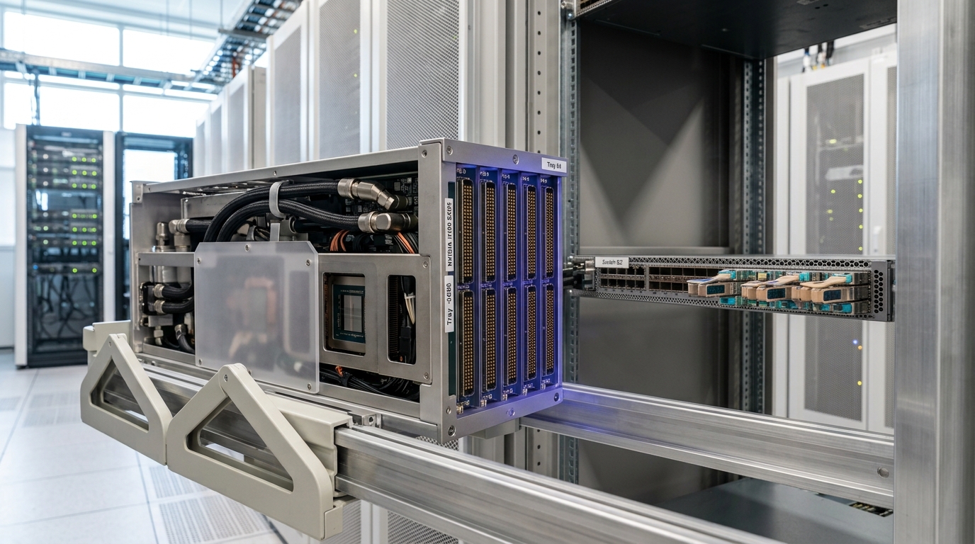
A compute tray mid-seating: the scale-up fabric lives on the backplane a few centimetres from the die; the scale-out fabric starts an arm's length away, at the rack's rear face. — Image prompt and art direction by Brecht Corbeel; generation pending.

Abstract

A large training job is not one computation; it is thousands of GPUs exchanging gradients and activations across two physically different fabrics stitched together at a chassis boundary. This article walks the mechanics: how a scale-up domain built on NVLink and NVSwitch differs from a scale-out fabric built on InfiniBand or RoCE Ethernet, how ring and tree all-reduce actually move bytes across a fat-tree or dragonfly topology, and why congestion and tail latency originate at specific, identifiable points in that topology rather than being a diffuse property of "the network." Every claim is tied to a vendor architecture document, a standards specification, or a systems paper, with vendor assertions and analytical inference marked as such.

A training run does not run on a GPU. It runs on thousands of them, and the sentence that actually describes what happens during a training step is not about floating-point throughput — it is about where a chunk of gradient data currently is: on a die, on a backplane a few centimetres away, or on an optical cable two rows over. Two physically different fabrics carry that chunk, built from different silicon, obeying different rules, and a training cluster’s real performance is set by the seam between them at least as much as by either fabric’s raw bandwidth.

This is a mechanics piece. It walks the scale-up fabric that lives inside a rack, the scale-out fabric that connects racks to each other, the collective operations that decide how data actually moves across both, the topologies that a scale-out fabric is built from, and the place — a specific, identifiable place, not a diffuse property of “the network” — where congestion and tail latency originate.

Two fabrics, not one

Scale-up is the fabric inside a single coherent domain: a set of GPUs that can address each other’s memory directly, at a bandwidth close to what a GPU uses to talk to its own DRAM. NVIDIA’s current generation of this is NVLink 5 paired with NVSwitch. A single Blackwell-generation GPU exposes up to eighteen NVLink connections at 100 gigabytes per second each, for roughly 1.8 terabytes per second of aggregate bandwidth per GPU — about fourteen times a PCIe Gen5 link [1]. That bandwidth only becomes usable at scale because of the switch: an NVSwitch chip is a dedicated crossbar that forwards NVLink traffic between GPUs without routing it through any GPU’s own compute path, and the GB200 NVL72 rack wires 72 Blackwell GPUs through a layer of these switches into what NVIDIA describes as a single non-blocking NVLink domain with 130 terabytes per second of aggregate bandwidth [1]. That is a vendor architecture claim, not an independent measurement, but it is a specific, falsifiable one: any GPU in that domain can reach any other at close to full NVLink bandwidth simultaneously with every other GPU doing the same, which is the actual definition of “non-blocking” in this context.

Scale-out is everything past that domain’s edge: the fabric that connects one NVL72 rack — or one HGX-class server — to the next, and the next, up to the size of the training job. This fabric is built from InfiniBand or from Ethernet carrying RDMA (RoCEv2), and it looks, mechanically, like a conventional data network: discrete packets, discrete switch chips, discrete queues, and routing decisions made hop by hop rather than one shared address space. InfiniBand’s architecture spans a full physical-through-transport stack defined by the InfiniBand Trade Association, and the IBTA’s most recent XDR generation targets 800 Gb/s-class per-port signaling specifically to keep pace with AI cluster growth [7] [8]. Meta’s alternative — RoCEv2 over a purpose-built Ethernet backend, kept physically and operationally separate from its general-purpose datacenter network — is documented in detail in a 2024 SIGCOMM paper describing clusters of thousands of GPUs each, coordinated over training jobs that run for weeks [4]. Both are legitimate, deployed answers to the same question — how do you move a gradient chunk between racks — and the disagreement between the InfiniBand and Ethernet camps in this industry is real and not a “true winner exists but is being obscured” situation: it is a genuine trade between an architecture purpose-built for RDMA lossless delivery and an architecture that reuses a much larger commodity Ethernet ecosystem and operational tooling. A newer, third position — the Ultra Ethernet Consortium’s Specification 1.0, published to make commodity Ethernet switch silicon behave like an AI-fabric transport at the protocol level — is discussed below in the congestion section, since that is exactly what it targets [2].

The mechanical distinction that matters is this: inside the scale-up domain, a GPU issuing a memory access to a peer’s memory does not construct a packet, does not consult a routing table per message, and does not wait behind another flow’s queue in the way a switched network’s port does — the NVSwitch crossbar is closer to a wide, dedicated bus than to a router. Past the domain’s edge, every one of those things happens. A training step’s communication cost is therefore not one number; it is the cost of moving data inside the domain (cheap, wide, low-latency) plus the cost of moving data across the domain boundary (governed by ordinary packet-switched network behavior) — and a job whose communication pattern crosses that boundary more than necessary pays the second cost far more often than a well-partitioned job needs to.

This is also why “scale-up” and “scale-out” are not merely marketing labels for “fast” and “slow” networks; they describe two different consistency and addressing models. A GPU inside an NVLink domain can issue a load or store against another GPU’s memory address and get a result back through the same coherence-adjacent path it would use locally — the NVSwitch fabric is designed so that software largely does not need to reason about which physical GPU currently holds a given piece of data, only which logical address it lives at. A scale-out fabric offers no such illusion: crossing it always means an explicit message, with an explicit source, destination, and completion signal, handled by an RDMA verb or a collective-library call rather than a plain memory access. Parallelism strategies in large model training are shaped directly by this difference. Tensor parallelism, which shards a single layer’s matrix multiplication across GPUs and requires an all-reduce or all-gather on nearly every layer, is normally kept entirely inside the scale-up domain precisely because its communication volume per step is too large and too frequent to survive crossing into scale-out territory at practical throughput. Data parallelism, which only needs to average gradients once per training step rather than once per layer, is the strategy usually pushed across the scale-out fabric between racks, because its coarser, less frequent communication pattern tolerates the added latency and queuing of a packet-switched hop. Pipeline parallelism sits in between, exchanging only activations and gradients at stage boundaries, and is often the parallelism dimension chosen specifically to straddle the domain boundary when a model’s parameter count exceeds what one scale-up domain can hold.

What a collective operation is actually doing

Distributed training does not send arbitrary messages; it runs collective operations — chiefly all-reduce (used to average gradients across all workers) and all-gather / reduce-scatter (used in sharded and pipeline-parallel setups). NVIDIA’s NCCL library is the collective-communication layer that most training stacks call into on top of both fabrics, and it does not use one algorithm for all situations — it selects among ring, tree (specifically a double-binary-tree construction), and switch-assisted collectives depending on message size and worker count, based on latency and bandwidth profiles NVIDIA measured on its own hardware [5].

The ring algorithm is the one worth understanding mechanically, because it is bandwidth-optimal and because its cost model exposes exactly why topology matters. In a ring all-reduce across p workers, each worker is logically placed on a ring; a gradient buffer of size S is split into p chunks, and each worker simultaneously sends one chunk to its ring-neighbor while receiving a different chunk from its other neighbor, reducing (summing) as chunks arrive. A complete all-reduce takes 2(p-1) such steps, each moving S/p bytes [5]. The total data volume any one worker sends over the whole operation is:

V = 2(p-1)\cdot\frac{S}{p} \approx 2S \quad \text{for large } p

which is the reason ring all-reduce is called bandwidth-optimal: in the limit, total traffic per worker approaches twice the buffer size regardless of how many workers participate, rather than growing with p. What does grow with p is the number of sequential steps, 2(p-1), and each step’s latency is bounded below by the slowest link and the slowest worker in the ring — which is precisely why NCCL switches to a tree algorithm for smaller messages and larger worker counts, trading some bandwidth efficiency for a \log p step count instead of a linear one [5]. This is an analytical property of the algorithm, not a vendor claim; the tree-versus-ring choice NCCL actually makes at runtime, however, is implementation-specific tuning NVIDIA has published as measured behavior on its own systems, and should be read as a vendor-characterized default rather than a universal law [5].

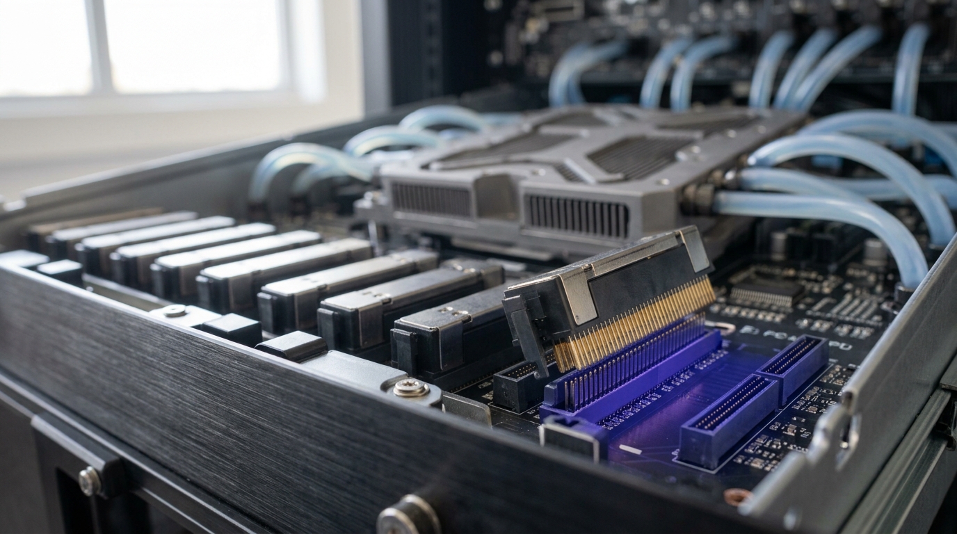
Figure 1. Scale-up mechanics: every GPU's NVLink lanes terminate on this backplane, and an NVSwitch chip forwards between them without ever leaving the tray. — Image prompt and art direction by Brecht Corbeel; generation pending.

The consequence for topology: a ring or a tree is a logical structure NCCL imposes on the workers, but every logical hop in that structure has to cross a physical link, and if that physical link crosses the scale-up/scale-out boundary, the hop’s cost changes by roughly an order of magnitude. Collective-communication libraries handle this by being topology-aware — preferring to complete as much reduction as possible inside a fast domain (using NVSwitch, in NVIDIA’s case) before crossing to the scale-out fabric — but the boundary cannot be made to disappear, only crossed as rarely as the parallelization strategy allows.

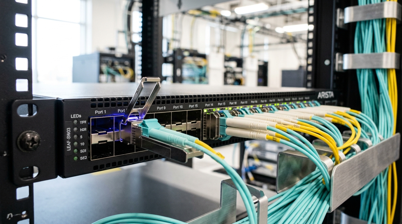
Figure 2. Scale-out mechanics: past the tray's edge, every hop is a discrete packet on a discrete cable, arbitrated by a switch queue rather than a shared memory fabric. — Image prompt and art direction by Brecht Corbeel; generation pending.

Topology: what a fat-tree and a dragonfly are actually solving

A scale-out fabric’s topology is not a stylistic choice; it is a statement about how many switches a worst-case message has to cross, and how much of the fabric’s total capacity is reserved for exactly that worst case. A Clos-derived fat-tree — the topology Google has run and progressively evolved in its own datacenter fabric since at least 2004, documented across its 2015 “Jupiter Rising” and 2022 “Jupiter Evolving” papers — connects racks through at least two stages of switches so that, with enough spine capacity, any rack can reach any other rack without the path being forced through a single bottleneck switch [9] [10]. Google’s own account of that decade of production experience quantifies what an evolving topology actually bought: a move from a fixed Clos toward a direct-connect topology among aggregation blocks, using optical circuit switches for dynamic reconfiguration, that the company reports delivered five times higher speed and capacity alongside a 30 percent capex reduction and a 41 percent power reduction over that period [10]. Those are Google’s own reported figures for its own fabric, not an independently audited benchmark, and they describe a hyperscale general-purpose network’s evolution rather than a purpose-built AI training fabric — but they are a specific, sourced data point on what topology change is actually worth, which is more than most industry claims about “the network” offer.

The dragonfly topology, introduced by Kim, Dally, Scott and Abts, takes a different structural bet, originally aimed at HPC interconnects rather than datacenter Ethernet fabrics. Instead of uniform multi-stage switching, it groups high-radix routers into virtual “super-routers” connected to each other by a smaller number of expensive, long global channels, so that a minimally routed packet crosses at most one global hop between groups [3]. The paper’s central argument is economic as much as architectural: since cabling — not switch silicon — dominates large interconnect cost, a topology should be judged by how few long cables it needs to reach a given diameter, and dragonfly was explicitly optimized against that constraint rather than against raw path diversity [3]. This is why dragonfly variants show up more often in HPC-derived AI clusters than fat-tree does, while fat-tree (and its Clos ancestors) dominates hyperscale training fabrics built on commodity Ethernet or InfiniBand switch silicon: the two topologies were optimized against different cost functions — cable count versus switch-stage uniformity — and neither is a strict subset of the other’s advantages. Where practitioners disagree is less about which topology is “better” in the abstract and more about which failure mode a given operator is more willing to accept — dragonfly’s global channels, if under-provisioned, create very specific highly-loaded links, while a fat-tree’s blocking behavior is more evenly distributed and depends heavily on the spine’s oversubscription ratio.

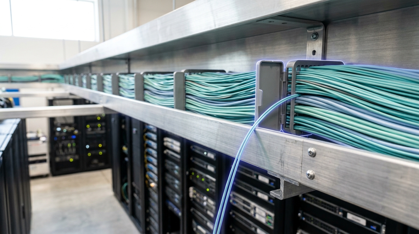
Figure 4. Every hop up a fat-tree or across a dragonfly's global links adds a queueing point; the topology is really a statement about how many of these convergence points a message must cross. — Image prompt and art direction by Brecht Corbeel; generation pending.

Where congestion actually starts

“Congestion” is often described as a property of a network in general; mechanically, it starts at a single point: an output queue on a switch port receiving traffic faster than that port can drain it. This is called incast when it happens because many senders converge on one receiver at once — exactly the traffic pattern a reduce-scatter or an all-gather produces, since many workers legitimately need to send to the same destination in the same short window. The queue fills, and once it does, every flow sharing that queue experiences added latency regardless of whether that flow’s own sender is misbehaving.

Data Center TCP, standardized as RFC 8257, was built specifically to address this: rather than waiting for a dropped packet to signal congestion (as classic TCP does), DCTCP has switches mark packets with Explicit Congestion Notification as queue occupancy crosses a threshold, and has the receiver reflect back the fraction of marked bytes so the sender can scale its window down proportionally to how congested the path actually is, rather than halving it on any single mark [6]. The RFC’s own stated result is that DCTCP sustains the same or better throughput than conventional TCP while using roughly 90 percent less switch buffer, specifically because it reacts to the degree of queue buildup rather than to a binary loss signal [6]. That figure is drawn from the specification’s own reported evaluation, not an independent third-party benchmark, and it describes general datacenter TCP traffic rather than AI-training RDMA flows specifically — but the mechanism (act on queue occupancy before loss, not after) is the same mechanism newer AI-fabric transports have since adopted and extended.

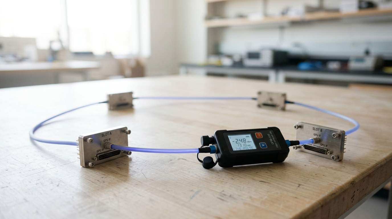
Figure 3. A ring all-reduce never touches every peer at once; a chunk of gradient moves one hop per step, and the ring's length sets the number of steps before it returns. — Image prompt and art direction by Brecht Corbeel; generation pending.

The Ultra Ethernet Consortium’s Specification 1.0, aimed explicitly at AI and HPC traffic on commodity Ethernet switch silicon, layers several additional mechanisms onto that same underlying problem: packet spraying across every available path rather than pinning a flow to one path, out-of-order delivery with reassembly handled at the NIC instead of requiring in-order arrival, packet trimming (forwarding a shortened header instead of silently dropping a full packet when a queue is full, so the receiver learns about congestion immediately instead of waiting for a retransmission timeout), and a receiver-driven credit scheme the spec calls Receiver Credit Congestion Control, designed specifically to manage incast by having the receiver — the party that can actually see all the converging senders — control the admission rate rather than each sender guessing independently [2]. This is a vendor-consortium characterization of its own specification rather than an independent measurement of deployed performance, and the specification is new enough that production deployment experience at the scale Meta or Google report for their own fabrics is not yet publicly documented. Notably, Meta’s own reported production choice for its RoCE fabric is not DCQCN-style proactive rate control at all: the SIGCOMM paper describes leaning primarily on Priority Flow Control (a link-level, non-proportional back-pressure mechanism) combined with receiver-driven admission logic built into its own collective-communication library, rather than the window-scaling ECN approach DCTCP popularized [4]. That is a real, reported divergence in practice between how the standards bodies frame congestion control and how at least one hyperscaler actually runs it in production, and it should be read as exactly that divergence rather than resolved into a single “how AI networks do congestion control” answer.

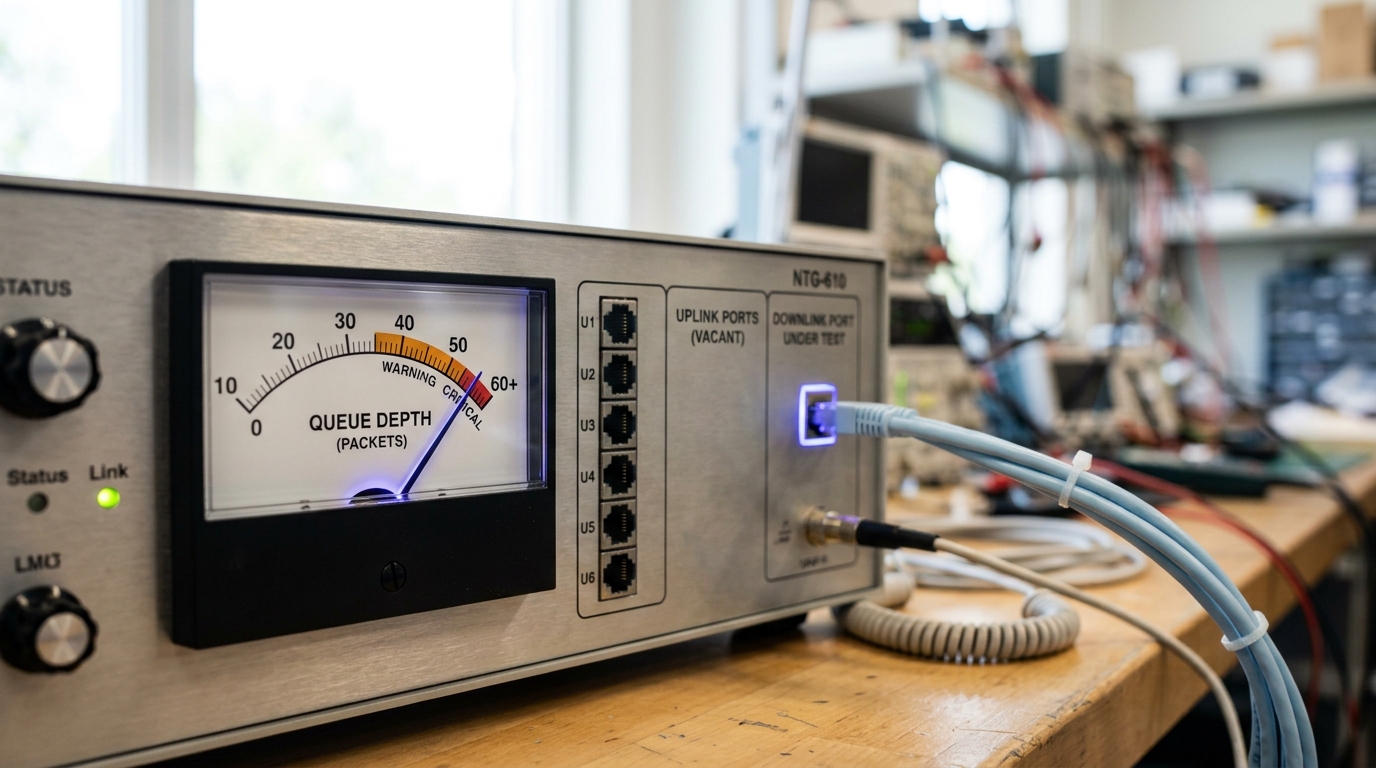
Figure 5. Congestion starts exactly here: many senders converge on one output port faster than it can drain, and the queue fills before any single link looks overloaded. — Image prompt and art direction by Brecht Corbeel; generation pending.

The seam is the argument

Put the pieces together and the picture that emerges is not “faster fabric wins.” It is that a training cluster is built from two fabrics with genuinely different physics — a coherent, switch-free memory-class fabric inside a rack, and a queued, packet-switched fabric between racks — bridged by a boundary that collective-communication software tries to cross as rarely as possible, sitting on top of a topology chosen for a specific cost trade-off (cable count versus stage uniformity), whose performance under real training traffic is set less by peak advertised bandwidth than by what happens at the specific ports where many senders converge on one receiver at the same moment. Every widely cited number in this space — NVIDIA’s 130 TB/s NVL72 domain, Google’s 5x capacity and 41 percent power figures, DCTCP’s 90 percent buffer reduction — is a claim from the party that built or specified the system being described, verifiable in its own published document but not independently replicated across vendors in a single comparable benchmark. Reading interconnect performance claims requires keeping that provenance attached to every figure, not averaging it away into a single cross-vendor ranking.

A bounded, falsifiable expectation for the next several years: as scale-up domains grow (NVIDIA’s own roadmap direction, per its published NVL72 architecture, is toward larger non-blocking domains rather than smaller ones), the scale-out fabric’s job increasingly narrows to exactly the traffic that cannot be kept inside a domain — meaning congestion-control sophistication at the domain boundary, not raw scale-out bandwidth, should be the more consequential lever on realized training throughput over roughly the next two to three years. The observable indicator would be published training efficiency (achieved-versus-theoretical FLOP/s at fixed cluster size) improving faster for clusters that adopt receiver-driven or credit-based congestion schemes (Ultra Ethernet-style, or Meta’s reported approach) than for otherwise-comparable clusters that do not. This would be disconfirmed if a hyperscaler publishes comparable training efficiency gains driven primarily by scale-out link-speed upgrades (e.g., a straight XDR InfiniBand or higher-radix Ethernet generation swap) with congestion control held constant — which would indicate raw scale-out bandwidth, not boundary-crossing congestion behavior, remains the binding constraint.

A note on what “actually work” leaves out

None of the mechanics above resolve into a single ranking of NVLink versus InfiniBand versus RoCE Ethernet, and that omission is deliberate rather than an oversight. These are not three competing answers to one question; they are answers to three different questions asked at three different points in the same cluster. NVLink and NVSwitch answer “how does a fixed, physically bounded group of GPUs share memory at close to local-memory bandwidth,” and that question has a hard physical ceiling set by how many GPUs one non-blocking crossbar generation can address, which is exactly why NVIDIA reports the NVL72 domain’s size (72 GPUs) as a fixed architectural property of one rack generation rather than a tunable parameter [1]. InfiniBand and RoCE Ethernet answer “how do an arbitrary and growing number of these bounded groups talk to each other,” and that question has no comparable hard ceiling — only the cost, in switches, cabling, and power, of adding another stage of fan-out — which is why both the IBTA and the Ultra Ethernet Consortium keep publishing new specification generations rather than declaring the scale-out problem solved [8] [2]. Treating these as substitutable, and asking which one “wins,” discards the information that actually explains a real cluster’s behavior: which of the two questions was the bottleneck for a specific job, on a specific day, at a specific point in its communication pattern. That is also why operators who build both kinds of fabric — Meta’s RoCE backend network kept deliberately separate from its general-purpose datacenter network is one documented example — treat the choice as an engineering trade evaluated against their own workload mix, not as a referendum on which standards body is correct [4].

Sources

1. NVIDIA. NVIDIA Contributes NVIDIA GB200 NVL72 Designs to Open Compute Project. NVIDIA Technical Blog (2024).
2. Ultra Ethernet Consortium. Ultra Ethernet Consortium (UEC) Launches Specification 1.0 Transforming Ethernet for AI and HPC at Scale. Ultra Ethernet Consortium (2025).
3. Kim, J.; Dally, W. J.; Scott, S.; Abts, D.. Technology-Driven, Highly-Scalable Dragonfly Topology. IEEE / ISCA 2008 (also IEEE Micro, 2009) (2008). DOI: 10.1109/ISCA.2008.19.
4. Meta (Engineering at Meta / SIGCOMM 2024). RDMA over Ethernet for Distributed AI Training at Meta Scale. ACM SIGCOMM 2024 (2024). DOI: 10.1145/3651890.3672233.
5. Various authors. Demystifying NCCL: An In-depth Analysis of GPU Communication Protocols and Algorithms. arXiv (2025).
6. Bensley, S.; Thaler, D.; Balasubramanian, P.; Eggert, L.; Judd, G.. Data Center TCP (DCTCP): TCP Congestion Control for Data Centers. IETF (2017).
7. InfiniBand Trade Association. InfiniBand Specification Frequently Asked Questions. InfiniBand Trade Association (2024).
8. InfiniBand Trade Association. IBTA Unveils XDR InfiniBand Specification to Enable the Next Generation of AI and Scientific Computing. InfiniBand Trade Association (2024).
9. Google. Jupiter Rising: A Decade of Clos Topologies and Centralized Control in Google's Datacenter Network. ACM SIGCOMM Computer Communication Review (2015). DOI: 10.1145/2829988.2787508.
10. Google. Jupiter Evolving: Transforming Google's Datacenter Network via Optical Circuit Switches and Software-Defined Networking. ACM SIGCOMM 2022 (2022). DOI: 10.1145/3544216.3544265.

Originally published at https://absolutedigitalpublishers.com/articles/how-ai-datacenter-interconnects-actually-works.