Comparing the Main Approaches to Scientific Instruments and Metrology
Electron microscopy, atomic force microscopy, and X-ray diffraction all resolve structure at atomic scale, but they trade resolution, sample survival, and generality against each other in ways no single ranking captures.
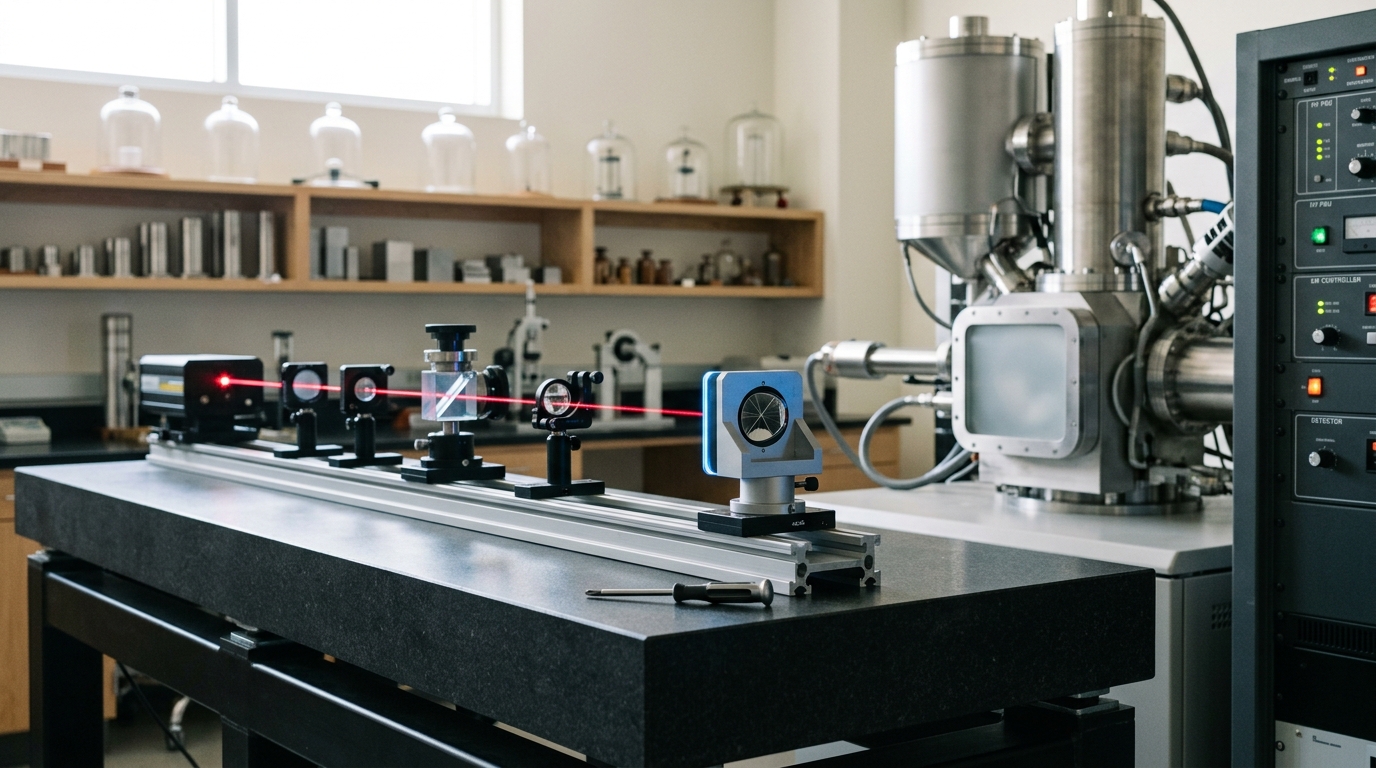
A national calibration laboratory: three measurement chains, one shared requirement — a traceable standard behind every reading. — Image prompt and art direction by Brecht Corbeel; generation pending.
Abstract
Every claim to have measured something rests on a chain: a calibrated instrument, a traceable standard, and a stated uncertainty. This article compares the major approaches to structural characterization at the smallest scales — transmission and scanning electron microscopy, atomic force microscopy, and X-ray diffraction and crystallography — on resolution, sample requirements, and destructiveness, then situates that comparison inside the metrology infrastructure (SI units, the GUM uncertainty framework, and the CIPM MRA interlaboratory comparison network) that makes any of their outputs comparable across laboratories at all. The approaches are complementary rather than competing: each answers a different question about the same specimen, and reproducibility across a field depends on traceability as much as on any single instrument's raw resolution.
Every number a scientific instrument reports is a claim about the world, and every claim rests on a chain most readers never see: a calibrated device, a standard the device was checked against, and a stated uncertainty bounding how much the reading might be wrong. Strip that chain away and the number is not measurement, it is opinion. The chain is what metrology — the science of measurement — exists to build and maintain, and it is the same infrastructure whether the instrument in question is a kitchen thermometer or a cryogenic diffractometer resolving a protein’s active site to better than two Angstroms.
This article compares the major instrumental approaches used to characterize structure at the smallest scales science currently probes routinely: transmission and scanning electron microscopy, atomic force microscopy, and X-ray diffraction and crystallography. These four are not rivals competing for one throne. They answer different questions about the same class of specimen, and a working structural-biology or materials-science lab typically uses several of them on the same sample in sequence. The comparison that matters is not “which is best” but “which trade-off does each one make, and along which axis.” Underneath that instrument-level comparison sits a second, quieter one: the international standards infrastructure — the International System of Units maintained by the Bureau International des Poids et Mesures (BIPM), the uncertainty framework in the Guide to the Expression of Uncertainty in Measurement (GUM), and the interlaboratory comparison network under the CIPM Mutual Recognition Arrangement (CIPM MRA) — that makes a resolution figure from one lab comparable to a resolution figure from another at all [1] [2] [4].
The measurement chain, before any instrument is chosen
A measurement is not merely a number; it is a number attached to a unit and an uncertainty. The SI Brochure defines the seven base units — the metre, kilogram, second, ampere, kelvin, mole, and candela — each now fixed by a defining constant of nature rather than a physical artifact, which is what lets a metre measured in one laboratory mean exactly the same length as a metre measured on another continent [1]. That definitional layer is necessary but not sufficient. A laboratory’s actual working instrument — an electron microscope’s magnification calibration, a diffractometer’s goniometer angle encoder, an AFM’s piezoelectric scanner — is calibrated against a chain of transfer standards that ultimately traces back to a primary realization of the relevant SI unit. This is the property called traceability, and it is what a Calibration and Measurement Capability (CMC) entry in the BIPM’s Key Comparison Database (KCDB) formally certifies: that a named national metrology institute’s calibration service for a given quantity has been peer-reviewed and found equivalent, within a stated uncertainty, to the other institutes participating in the CIPM MRA [5] [4].
Uncertainty itself has a standard grammar, laid out in the GUM and adopted domestically by NIST in Technical Note 1297. Every source of doubt about a measured value is classified as either a Type A evaluation — estimated from the statistical scatter of repeated observations — or a Type B evaluation — estimated from any other information, such as a calibration certificate, a manufacturer’s specification, or physical reasoning about a known systematic effect [2] [3]. These component uncertainties are combined, following an explicit propagation rule, into a combined standard uncertainty, which is then multiplied by a coverage factor (conventionally k=2, corresponding loosely to a 95% confidence interval under a normal-distribution assumption) to produce the expanded uncertainty that actually gets reported alongside a result [3]. If a resolution or a measured lattice spacing is quoted without an accompanying uncertainty, the number cannot be compared against another laboratory’s figure, however precise the instrument sounds. The combined standard uncertainty u_c(y) for a measured quantity y = f(x_1, x_2, \ldots, x_N) that is a function of several independently uncertain inputs is, to first order,
u_c^2(y) = \sum_{i=1}^{N} \left( \frac{\partial f}{\partial x_i} \right)^2 u^2(x_i)
which is the law of propagation of uncertainty the GUM formalizes [2]. This equation matters here because it is the reason a headline resolution figure for any of the four instruments below is an idealized best case: it is the quadrature sum over every contributing uncertainty (mechanical drift, detector noise, calibration-standard uncertainty, vibration) and any single dominant term — often sample or environmental, not the instrument’s fundamental physics — can set the practical floor well above the textbook number.
Structural characterization: four approaches, one question asked four ways
The shared question these four approaches address is “what is the arrangement of atoms or features in this specimen, and at what scale.” Each answers it with a completely different physical interaction, and that choice of interaction determines a bundle of consequences — achievable resolution, how much sample preparation is required, whether the specimen survives, and what kind of specimen the technique can even accept.
Transmission electron microscopy: atomic columns, at a cost
Transmission electron microscopy (TEM) fires a focused beam of high-energy electrons through an extremely thin specimen and forms an image from the electrons that pass through, exploiting the fact that an electron’s de Broglie wavelength at typical TEM accelerating voltages is thousands of times shorter than the wavelength of visible light. That short wavelength is what lets TEM resolve individual atomic columns — a resolution regime unreachable by any light-based instrument [6]. The price is steep and structural: a conventional TEM specimen must be thinned to under roughly 100 nanometres so the beam can pass through it at all, and preparing that thin section is itself a nontrivial procedure specific to the material — ultramicrotome sectioning and heavy-metal staining for biological tissue, mechanical polishing and ion milling or focused-ion-beam preparation for hard materials [6]. The interaction that produces the image is also what damages the specimen: a high dose of electrons deposits energy that can destroy fine structural detail during imaging itself, which is why beam-sensitive materials are imaged under deliberately reduced, “low-dose” conditions that trade signal for survivability [6]. TEM, in short, buys the highest attainable resolution in this comparison by requiring a destructively thinned sample and tolerating some unavoidable beam damage during the very act of looking.
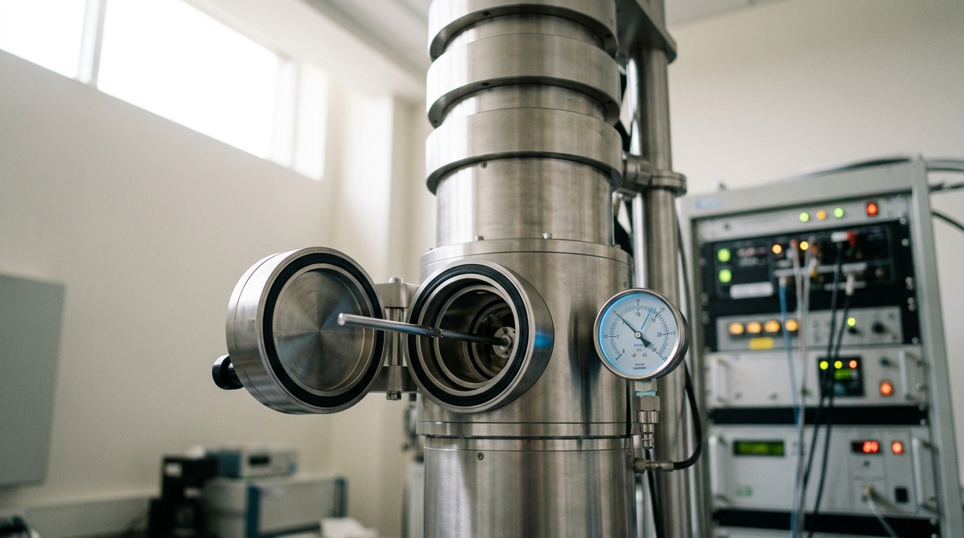
Figure 1. TEM resolves atomic columns, but the beam that forms the image also damages the specimen it strikes. — Image prompt and art direction by Brecht Corbeel; generation pending.
Scanning electron microscopy: the surface, mostly intact
Scanning electron microscopy (SEM) also uses an electron beam, but rasters it across a bulk specimen’s surface and forms an image from the secondary and backscattered electrons the surface emits, rather than from electrons transmitted through it. That difference in geometry is the whole story: SEM does not need an ultrathin section, so it can image a bulk, three-dimensional specimen’s surface topology directly. Point resolution in a well-configured instrument can reach roughly 0.4 nanometres, though most conventional instruments operate in the sub-nanometre to twenty-nanometre range — markedly coarser than TEM’s atomic-column resolution, because SEM is reading surface-emitted electrons rather than a transmitted diffraction pattern [7]. Non-conductive specimens typically need a thin conductive coating (gold, gold-palladium, platinum, or similar) sputtered on before imaging, and conventional SEM requires a high vacuum, which forces biological or wet samples to be dried or frozen first — environmental SEM variants relax this at the cost of some resolution and contrast [7]. Critically, though, the SEM interaction itself is essentially non-destructive: the beam’s electrons scatter from the surface without altering it, which is exactly why SEM is the instrument of choice for forensic evidence and irreplaceable artifacts that cannot be sacrificed to answer a structural question [7]. SEM trades TEM’s finest resolution for a specimen that survives the session largely unchanged.
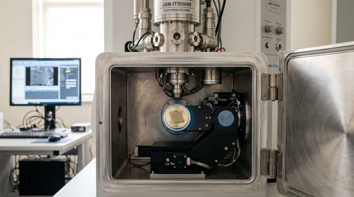
Figure 2. SEM trades TEM's atomic resolution for an intact surface: samples survive the imaging, coated or not. — Image prompt and art direction by Brecht Corbeel; generation pending.
Atomic force microscopy: touch, not radiation
Atomic force microscopy (AFM) abandons electromagnetic and electron-beam probing altogether and instead drags — or lightly taps — a nanometre-scale mechanical cantilever tip across a surface, inferring topography from the tiny deflections of the cantilever as short-range forces between tip and sample vary. Demonstrated resolution reaches fractions of a nanometre, and under the right conditions AFM resolves true atomic-scale features, putting its best case in the same regime as TEM despite the completely different physical mechanism [8]. AFM’s structural advantage over both electron techniques is sample compatibility: it requires no special coating that would irreversibly alter the specimen, and most operating modes work in ambient air or even in liquid, so no vacuum chamber is needed at all — a materials scientist can watch a process happen in real time in solution, something neither TEM nor conventional SEM can do [8]. Destructiveness is mode-dependent rather than fixed: tapping mode reduces damage relative to contact mode by keeping tip-sample contact brief and reducing lateral shear forces, but contact mode can still degrade soft biological samples through strong adhesive capillary forces during scanning [8]. AFM, then, occupies an unusual position in this comparison — matching the electron techniques’ best-case resolution while requiring the least sample preparation of the three, at the cost of imaging only a surface, one point of physical contact at a time, which makes large-area scans comparatively slow.
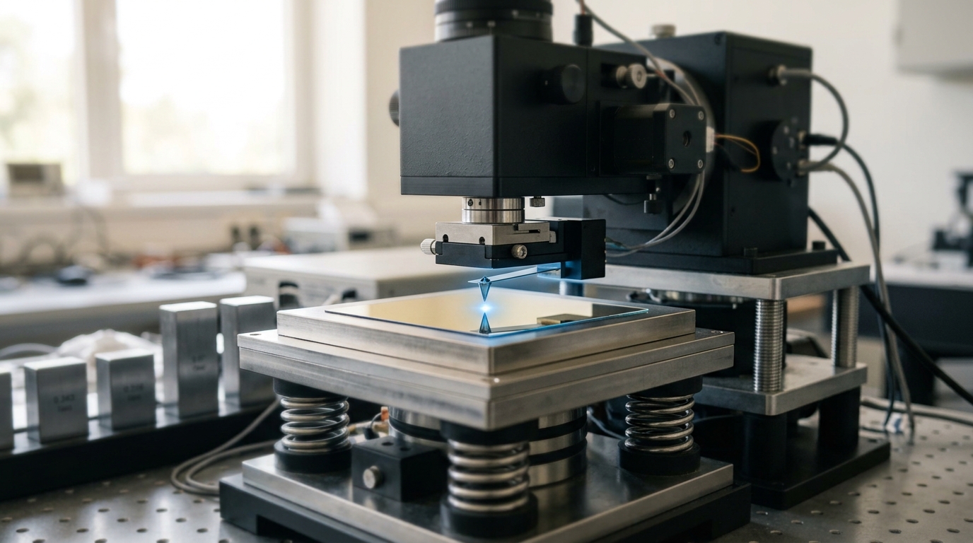
Figure 3. AFM needs no vacuum and no coating, only a cantilever tip a few nanometres wide brought close enough to feel the surface. — Image prompt and art direction by Brecht Corbeel; generation pending.
X-ray diffraction and crystallography: the whole lattice, if you can grow one
X-ray diffraction and crystallography ask a fundamentally different kind of question than the three imaging techniques above: rather than forming a real-space image point by point, a crystal is exposed to a beam of X-rays and the pattern of constructive interference — the diffraction pattern — is recorded and mathematically inverted to reconstruct the electron density, and from that the atomic positions, throughout the crystal’s repeating unit cell. Because the technique reads out an entire periodic lattice simultaneously rather than scanning it point by point, well-diffracting crystals routinely yield atomic-resolution structures, with individual atoms and chemical bonds appearing as identifiable features in the reconstructed electron-density map [9]. The requirement this technique cannot avoid is structural rather than instrumental: it needs a crystal, typically at least around a tenth of a millimetre in each dimension, pure in composition and free of significant internal defects such as cracking or twinning — and for many biological macromolecules, simply growing a crystal that diffracts well is the single hardest and most time-consuming part of the entire experiment [9]. X-ray exposure is also cumulatively destructive: radiation damage accumulates during data collection, which is why protein crystals are routinely flash-frozen in liquid nitrogen before and during exposure, a step that suppresses both radiation damage and thermal motion, and why some datasets must be merged from several crystals when any single one degrades too far to finish the job [9]. X-ray diffraction offers a global, whole-lattice readout that the point-by-point techniques cannot match in a single exposure, in exchange for a specimen requirement — a real, well-ordered crystal — that many materials of interest simply cannot satisfy.
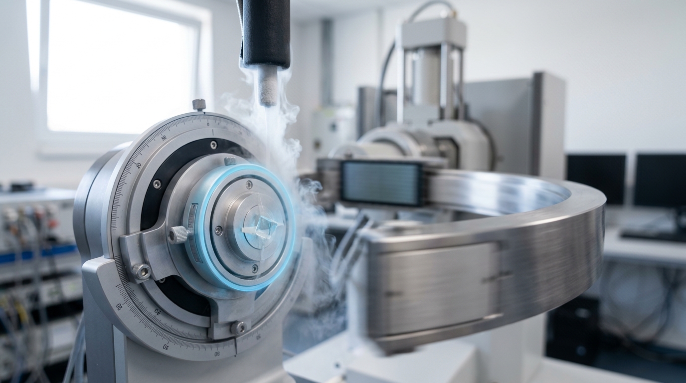
Figure 4. X-ray diffraction reads a crystal's whole lattice at once, at the cost of needing a crystal in the first place. — Image prompt and art direction by Brecht Corbeel; generation pending.
Reading the comparison honestly
Laid side by side on the three dimensions the assignment asks about: TEM offers the finest routine resolution but is destructive to a beam-sensitive specimen and demands an ultrathin section; SEM sacrifices atomic resolution for a largely non-destructive look at a bulk surface with modest preparation; AFM matches the best-case resolution of the electron techniques with the least preparation and no vacuum, at the cost of scan speed and a surface-only view; X-ray diffraction reads an entire lattice at once with excellent resolution but only when a suitable crystal exists, and its own probe accumulates damage over the exposure. None of these orderings survives being collapsed into a single “best instrument” ranking — a structural biologist solving a novel protein fold, a materials scientist watching corrosion progress in real time in a liquid cell, and a semiconductor fab inspecting a wafer’s surface defects are asking different questions, and each reaches for the instrument whose particular trade-off fits the question, often using two or three of these techniques on the same specimen in sequence to cross-validate what any single one alone could not confirm.
Detector technology sits underneath all four techniques as a further comparison worth naming, though it does not receive its own instrument-family treatment here: a diffractometer’s resolution and an electron microscope’s contrast both depend on the detector converting a physical signal (a photon, an electron) into a countable, calibrated digital value, and that detector’s own quantum efficiency, noise floor, and linearity are themselves subject to the same GUM-style uncertainty budgeting as the instrument as a whole [3]. A structural result is never better than the weakest calibrated link between the physical interaction and the number that leaves the software.
What “resolution” actually means across these four instruments
A subtlety worth making explicit: the word “resolution” is not measuring the same thing in each of the four techniques above, which is precisely why a naive numerical ranking across them is misleading. In TEM and SEM, resolution describes the smallest separation between two point-like features the optics can distinguish, fundamentally set by the electron wavelength and the lens aberrations of the column. In AFM, the relevant limit is a convolution of the true surface topography with the physical geometry of the cantilever tip itself — a blunter tip broadens every feature it scans regardless of the piezo scanner’s positional precision, so AFM’s headline sub-nanometre figures assume a tip sharp enough that this convolution effect is negligible, an assumption that degrades as tips wear during use [8]. In X-ray crystallography, “resolution” refers to the highest-angle diffraction spots still measurably above background, expressed in Angstroms of d-spacing under Bragg’s law, and it is a property of how well-ordered the crystal is — how few molecules in it are misaligned relative to their neighbors — at least as much as it is a property of the X-ray source or detector [9]. Comparing a TEM’s “0.1 nanometre” to a crystal structure’s “1.5 Angstrom resolution” as though they were entries on the same scale conflates an optical resolving-power limit with a statement about crystalline order; both are real and both are useful, but they answer different underlying questions and neither displaces the value of the other.
Interferometry, gravitational-wave detectors, and the extreme end of precision
The instruments above resolve structure at short length scales. A different family of instruments — laser interferometers — pushes precision along a single dimension (typically a length or a phase difference) to an extreme that has little to do with spatial resolution in the microscopy sense. Ground-based gravitational-wave interferometers are the sharpest publicly documented example: designed to detect a fractional change in arm length, expressed as strain, as small as roughly $h \approx 5 \times 10^{-22}$ — a distortion far smaller than a proton’s diameter integrated over a kilometers-long arm [10]. Reaching that sensitivity is a story about noise budgeting rather than a single dominant limitation: shot noise from the random arrival of photons in the laser beam limits sensitivity at high frequencies, while seismic noise and other environmental vibration dominate at low frequencies, and thermal noise from Brownian motion in mirror coatings sets a further floor in between [10]. Non-stationary disturbances — mechanical creaks, lightning, and other transient environmental events — must be identified and excluded through analysis before any candidate signal can be treated as a genuine detection rather than an instrumental artifact [10]. This is the same measurement-chain discipline described above, applied at an extreme: no single number describes “the sensitivity” without specifying the frequency band and the noise source assumed dominant in that band, exactly as a microscope’s resolution figure is meaningless without specifying the operating mode and sample conditions that number assumed.
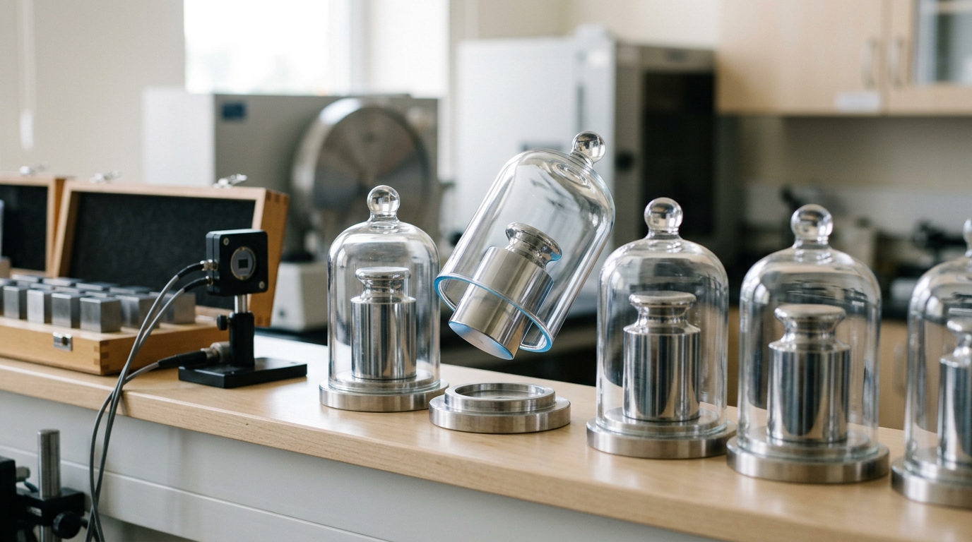
Figure 5. Traceability is a physical chain: every working instrument answers, through a series of transfer standards, to one of these. — Image prompt and art direction by Brecht Corbeel; generation pending.
Fact, vendor claim, analysis, and where this comparison should not go
Separating registers matters here because instrument marketing routinely blurs them. It is a fact, documented in peer-reviewed and standards-body sources, that TEM resolves atomic columns, that AFM resolution reaches fractions of a nanometre under favorable conditions, that SEM is comparatively non-destructive, and that X-ray crystallography requires a diffracting crystal [6] [8] [7] [9]. It is a vendor or manufacturer claim, not independently re-verified in this article, whenever a specific instrument model’s datasheet states a headline resolution number — such figures describe a best-case configuration under ideal alignment and sample conditions, and the GUM’s own propagation logic explains why the number achieved in a working laboratory on a real specimen is routinely coarser [2] [3]. It is analysis, not fact, to say that these four techniques are complementary rather than substitutable — that conclusion follows from comparing their trade-offs as laid out above, but it is an interpretive judgment about how the techniques are actually used together in practice, not a citable finding from any single source.
No scenario or prediction is offered in this article: the comparison above describes standing, already-realized capabilities and a well-documented uncertainty framework, not a forecast about how any of these techniques will change. Where a claim might have tempted a ranking — “the best instrument for structural biology,” “the most precise microscope” — that framing has been avoided deliberately, because the comparative dimensions above (resolution, sample requirements, destructiveness) trade against each other differently depending on the specimen and the question being asked, and reasonable practitioners choose differently among these tools for exactly that reason. The CIPM MRA’s interlaboratory comparison system exists for a related but distinct reason: not to declare one national laboratory’s calibration “better” than another’s, but to establish, through repeated blind comparison measurements circulated among institutes, that their results agree within their stated uncertainties — which is the operational definition of two measurements meaning the same thing [4] [5]. That discipline, more than any single instrument’s raw resolution figure, is what allows a measurement made in one laboratory to be trusted, checked, and reproduced in another.
Reproducibility begins in the calibration chain, not the analysis
A recurring diagnosis of reproducibility problems across experimental science places the failure downstream, in statistical analysis or publication incentives. That diagnosis is not wrong, but it skips a prior layer: a result cannot be reproduced by a second laboratory if the first laboratory’s instrument was never traceably calibrated in the first place, because there is then no shared reference against which either laboratory’s number can be checked. The SI’s redefinition around fixed physical constants, the GUM’s shared vocabulary for uncertainty, and the CIPM MRA’s network of key comparisons are the parts of the reproducibility problem that are solved before an experiment is even designed [1] [2] [4]. None of that infrastructure determines which structural-characterization instrument a given experiment should use — that choice still depends on the resolution, sample, and destructiveness trade-offs compared above — but it is the reason a resolution or lattice-spacing figure reported by one laboratory can be meaningfully compared, at all, against a figure reported by another using a different instrument on a different continent.
Sources
- Bureau International des Poids et Mesures. The International System of Units (SI Brochure), 9th edition. BIPM (2019).
- Joint Committee for Guides in Metrology. Evaluation of Measurement Data — Guide to the Expression of Uncertainty in Measurement (GUM), JCGM 100:2008. BIPM/JCGM (2008).
- Barry N. Taylor, Chris E. Kuyatt. Guidelines for Evaluating and Expressing the Uncertainty of NIST Measurement Results. NIST (1994).
- Bureau International des Poids et Mesures. The CIPM Mutual Recognition Arrangement (CIPM MRA). BIPM (2024).
- Bureau International des Poids et Mesures. KCDB — BIPM Key Comparison Database. BIPM (2026).
- Wikipedia contributors. Transmission electron microscopy. Wikimedia Foundation (2026).
- Wikipedia contributors. Scanning electron microscope. Wikimedia Foundation (2026).
- Wikipedia contributors. Atomic force microscopy. Wikimedia Foundation (2026).
- Wikipedia contributors. X-ray crystallography. Wikimedia Foundation (2026).
- Wikipedia contributors. Interferometric gravitational-wave detector. Wikimedia Foundation (2026).
Originally published at https://absolutedigitalpublishers.com/articles/comparing-the-main-approaches-to-scientific-instruments-and-metrology.