Comparing the Main Approaches to AI Inference Economics

Five largely independent decisions set what a token costs: hosting, architecture, capacity commitment, precision, and whether an answer can wait. This compares them and says plainly where the evidence supports a ranking and where it does not.

Self-hosted, API-based and managed inference are not one product priced three ways; each is a different transfer of ownership, risk and engineering burden. — Image prompt and art direction by Brecht Corbeel; generation pending.

Abstract

This article compares the main approaches available for procuring and serving AI inference by treating cost as the output of five largely independent choices rather than one market: who owns the accelerators a model runs on, whether the model activates all of its parameters per token or only a subset, how compute capacity is contracted, what numeric precision the weights run at, and whether a request is answered immediately or queued. For each axis it reports what providers and researchers have actually published about cost and performance tradeoffs, using verified pricing pages, systems papers and energy data rather than vendor marketing claims, and it works out the one piece of arithmetic — a break-even utilization rate for reserved capacity — that turns a published discount into a buyer-specific answer. It is explicit throughout about where a clean head-to-head ranking is possible and where the workloads, hardware generations and contract terms being compared are different enough that forcing a ranking would manufacture a result the evidence does not support.

The five decisions hiding inside “how much does inference cost”

Ask what it costs to serve a language model and the honest answer is that the question is underspecified in at least five separate ways before a number can mean anything. Whoever is asking has already made, or is about to make, five largely independent choices: who owns the accelerators the model runs on; whether the model activates all of its parameters on every token or only a fraction of them; whether the compute backing a request is bought at a spot price, an on-demand price, or under a reserved commitment; what numeric precision the weights and activations run at; and whether the request is answered the instant it arrives or held until capacity is free.

Each of these choices is documented separately, by a different kind of source — cloud pricing pages, GPU-cloud rate cards, architecture papers, quantization papers, hardware vendor specifications. None of them documents the others. A paper reporting a quantization speedup does not report what happens when the same technique is combined with mixture-of-experts routing on spot capacity; a cloud provider’s on-demand rate card does not report what a comparable workload would cost self-hosted, because self-hosting is not a product with a rate card at all. This article works through each axis in turn, reports what is actually published about its cost and performance tradeoffs, and stays deliberately explicit about the point at which the evidence stops supporting a ranking and a reader would have to compare workloads, hardware generations and contract terms that are not, in fact, the same thing.

Three ways to buy the compute behind a token

At the top level there are three structurally different ways an organisation gets language-model inference done, and they differ in what is being bought, not merely in price.

Self-hosted or colocated inference means the buyer owns or leases physical accelerators — in owned data-center space or in a colocation facility — and runs its own serving stack against them. The buyer carries utilization risk directly: an accelerator sitting idle overnight is capital that earned nothing that night, and the full engineering burden of batching, scheduling and keeping the fleet fed with work falls on the buyer’s own team. Amazon’s P5 instance family gives a concrete sense of the unit being bought: a p5.48xlarge configuration carries eight H100 GPUs with 640 gigabytes of aggregate HBM3 memory, and AWS states the generation delivers “up to 4x the performance of previous-generation GPU-based EC2 instances” and can “reduce cost to train ML models by up to 40%” — a training-cost claim from the vendor, not an inference-cost figure, and stated here as exactly that [5].

API-based inference means paying a foundation-model provider per token, with no visibility into the underlying hardware, batch size or utilization at all. OpenAI’s and Anthropic’s rate cards for their current model families are representative. As verified on 16 August 2026, OpenAI lists gpt-5.6-sol at 5 dollars per million input tokens and 30 dollars per million output tokens, gpt-5.6-terra at 2 and 12 dollars, and gpt-5.6-luna at 0.20 and 1.20 dollars [10]. Anthropic lists Claude Opus 5 at 5 dollars input and 25 dollars output per million tokens over the same period [9]. Here the provider absorbs utilization risk and the engineering burden of serving; the buyer pays a price that already has both baked in and cannot see the components separately.

Serverless or managed inference platforms sit structurally between the two: a third party operates the accelerators and the serving stack, as in the API case, but the buyer can typically choose between per-token serverless pricing and a dedicated allocation of capacity, as in the self-hosted case, without owning any hardware. Together AI’s rate card, verified 16 August 2026, makes the boundary visible inside a single vendor: the platform offers per-token serverless pricing for open-weight models, a dedicated-endpoint tier billed by the GPU-hour at 5.49 to 8.99 dollars on demand with reserved terms available by contacting sales, and a provisioned-throughput tier billed at 0.05 dollars per unit-minute with model-specific throughput guarantees, and states plainly that “most teams start with serverless inference and move to dedicated endpoints at scale” [8]. Microsoft’s Foundry Models documentation describes the same structural split inside Azure: a standard pay-per-token deployment with no latency guarantee, a priority-processing tier at a higher per-token rate with a defined latency target, a provisioned-throughput deployment billed hourly per unit “regardless of the number of tokens consumed” with its own latency service-level agreement, and a discounted batch tier for asynchronous work — four deployment types differing in billing unit and latency guarantee, on the same underlying models [7].

A genuine head-to-head between these three is harder than it looks, and it is worth being explicit about why. A self-hosted fleet’s real cost per token depends on a utilization rate that is a property of the buyer’s own traffic, not of the hardware; the same rack running at 20 percent utilization and 80 percent utilization produces very different costs per token from identical capital. An API price is a single number that has already absorbed the provider’s own utilization, model architecture and serving-stack choices, none of which the buyer can independently verify. A managed platform’s per-token serverless rate and its per-GPU-hour dedicated rate are not prices for the same product either — the dedicated rate buys guaranteed, unshared capacity, while the serverless rate buys a share of a multi-tenant pool whose price already reflects the provider’s success at keeping that pool busy with other customers’ traffic. Comparing a self-hosted total cost of ownership to a published API rate, without knowing the self-hosted fleet’s realized utilization, produces a number that looks like a comparison and is not one.

Self-hosted and colocated deployments are the one procurement approach where the buyer sees the electricity bill directly rather than having it folded into a vendor’s per-token rate, and the scale of that bill is now documented at the industry level. The International Energy Agency’s Energy and AI report states that data centers consumed approximately 415 terawatt-hours of electricity in 2024, about 1.5 percent of global electricity consumption, and that this demand has grown roughly 12 percent per year since 2017 — more than four times the growth rate of total electricity consumption — naming AI as “the most important driver of this growth” and projecting demand to reach approximately 945 terawatt-hours by 2030 [17]. That is an industry-wide figure, not a per-token cost, and it says nothing about any single deployment’s economics; what it establishes is that the power line item a self-hosted operator manages directly is a fast-growing and material fraction of a data center’s total cost, in a way that is invisible on a per-token invoice from an API provider.

Dense and mixture-of-experts models have different serving cost profiles

A second, largely independent axis is architectural: does the model activate every parameter on every token (dense), or does it route each token through a subset of “expert” sub-networks (mixture-of-experts, or MoE)?

The mechanism is documented across several public model families. Mixtral, an 8-expert sparse model, holds 47 billion total parameters but activates only 13 billion of them per token, using a router that selects 2 of its 8 experts per layer per token; its authors report that the resulting model matches or outperforms the dense 70-billion-parameter Llama 2 on the benchmarks they evaluated [12]. DeepSeek-V3 pushes the same idea further: 671 billion total parameters, of which only 37 billion are activated per token, combined with a multi-head latent attention mechanism and an auxiliary-loss-free load-balancing strategy, with pretraining reported to complete in 2.788 million H800 GPU-hours [11]. The foundational account of why this works is the Switch Transformer paper, which frames sparse routing as selecting “different parameters for each incoming example,” producing “a sparsely-activated model — with outrageous numbers of parameters — but a constant computational cost,” and reports pretraining 7 times faster than dense T5-Base and T5-Large at matched compute, and 4 times faster than the larger T5-XXL when scaled toward a trillion parameters [13].

For inference cost specifically, what matters is that per-token compute tracks activated parameters, not total parameters. Approximating compute per token as proportional to the parameter count actually touched [13, 11], the ratio of dense to MoE compute at equal activated size is approximately

\frac{C_{\mathrm{dense}}}{C_{\mathrm{MoE}}} \approx \frac{N_{\mathrm{dense}}}{N_{\mathrm{active}}}

for a dense model with N_{\mathrm{dense}} parameters compared against an MoE model activating N_{\mathrm{active}} of its N_{\mathrm{total}} parameters per token. What this ratio hides is exactly what a compute-only comparison always hides: memory. Serving an MoE model requires holding all N_{\mathrm{total}} parameters resident — on one device or, more often, sharded across several with communication between them whenever a batch’s tokens route to different experts — even though only N_{\mathrm{active}} of them do arithmetic on any given token. A dense model of the same activated size carries no such requirement. The compute saving is real and is the reason MoE models can be commercially attractive to serve; the memory and networking cost it trades against is equally real, and neither the Switch Transformer paper, the Mixtral paper nor the DeepSeek-V3 report discloses enough about any specific production serving stack to say where the net trade lands for a given deployment.

One place this tradeoff becomes visible from outside is a rate card that prices both architectures for the same buyer. Together AI’s serverless pricing, verified 16 August 2026, lists DeepSeek V4 Flash at 0.14 dollars input and 0.28 dollars output per million tokens and DeepSeek V4 Pro at 1.74 dollars input and 3.48 dollars output, against 1.04 dollars flat for the dense Llama 3.3 70B [8]. Read as a data point, that is real: it shows one operator pricing sparse and dense models differently on shared infrastructure. Read as a ranking, it is not usable, because DeepSeek V4 Flash, DeepSeek V4 Pro and Llama 3.3 70B are not the same capability at three prices — they are three different models with different total and active parameter counts, different training data and different quality on any given task, so a lower headline rate for one is not evidence that mixture-of-experts serving is cheaper in general. It is evidence that one vendor priced these particular models this way.

Figure 1. A mixture-of-experts model pays compute for a handful of active parameters per token but still pays memory for all of them; a dense model pays both costs on every token. — Image prompt and art direction by Brecht Corbeel; generation pending.

On-demand, reserved and spot capacity are different products, not different prices

The same physical accelerator can be bought under at least three commitment structures, and providers offering all three are explicit that they are not variations on one price.

On-demand capacity carries no commitment: AWS describes EC2 on-demand instances as letting a buyer “pay for compute capacity by the hour or second… with no long-term commitments” [1]. It is the most flexible and, per unit of compute actually used, typically the most expensive of the three.

Reserved or committed capacity trades a forward commitment for a lower rate. AWS’s Compute Savings Plans and EC2 Instance Savings Plans, verified 16 August 2026, require a 1-year or 3-year commitment expressed in dollars-per-hour of usage, in exchange for discounts of up to 66 percent and up to 72 percent respectively off on-demand rates, with usage beyond the committed amount reverting to standard on-demand pricing [4]. Reserved commitments built around inference throughput specifically work the same way structurally: Microsoft’s Foundry Models documentation describes provisioned-throughput deployments billed hourly per unit “regardless of the number of tokens consumed,” with the meter running from deployment creation until deletion, and Azure Reservations offering a discounted effective rate on that meter for a 1-month or 1-year commitment — while stating explicitly that “reservations don’t guarantee capacity” and that a deployment must first confirm capacity is available before the reservation is purchased [7]. Together AI’s dedicated-endpoint and provisioned-throughput tiers, billed by the GPU-hour or by the throughput-unit-minute with reserved terms negotiated directly, follow the same shape on a third platform [8].

Spot or preemptible capacity goes the other direction: the buyer accepts that the provider can reclaim the capacity at short notice, in exchange for a much steeper discount. AWS states that Spot Instances are “available at a discount of up to 90% off compared to On-Demand pricing,” and that the historical average interruption frequency “across all Regions and Instance types” has been under 5 percent, though published guidance breaks actual rates into bands from under 5 percent up to over 20 percent depending on the specific instance type and region, recommending diversification across types and availability zones precisely because the rate is not uniform [2, 3]. A GPU-focused cloud provider shows the same structure at accelerator-specific prices: CoreWeave’s published rate card, verified 16 August 2026, lists an 8-GPU H100 node at 49.24 dollars per hour on demand and 19.71 dollars per hour on spot pricing — close to a 60 percent discount — with committed-usage discounts of up to 60 percent available for buyers willing to negotiate a reserved term directly [6].

Figure 2. Reserved capacity is a discount purchased with a forward commitment, not a lower price for the same product; it only pays off above a utilization threshold the buyer alone knows. — Image prompt and art direction by Brecht Corbeel; generation pending.

Here the break-even arithmetic is genuinely simple, and worth writing down, because it is the one place in this comparison where a clean model — not a ranking of vendors — is possible. Let a reserved commitment cost P_r per accelerator-hour, and let the on-demand or serverless rate that would otherwise serve the same throughput cost P_d per accelerator-hour at full utilization. If the buyer’s realized utilization of the reserved capacity is u \in (0, 1], the reserved option is cheaper exactly when

P_r < u \cdot P_d, \qquad \text{i.e.} \qquad u > \frac{P_r}{P_d} \equiv u^{*}.

Below the break-even utilization u^{*}, paying on demand only for the hours actually used is cheaper than holding a reservation that sits partly idle; above it, the reservation wins. What no published rate card can supply is u itself — a property of the buyer’s own traffic, not of any vendor’s pricing page — which is exactly why “is reserved capacity worth it” has no answer that holds across buyers, only a formula that turns a buyer’s own utilization forecast into one.

Spot capacity adds a second variable the formula above leaves out: the cost of interruption. A workload that can checkpoint and resume, or tolerate being requeued elsewhere, converts a 60- to 90-percent discount into nearly pure savings [2, 6]. A workload serving live, synchronous requests generally cannot absorb an unannounced loss of its serving capacity without a user-visible failure, which is why spot capacity appears in inference procurement mainly for offline, batchable or easily-rerouted work rather than for latency-sensitive serving — a distinction the batch-versus-real-time comparison below develops directly.

Figure 3. Spot capacity trades a steep discount for the provider's right to reclaim it without warning; whether that trade pays off depends on whether the workload can absorb the loss. — Image prompt and art direction by Brecht Corbeel; generation pending.

Precision is a serving decision that trades cost against quality at the same time

Every other axis in this comparison changes what a request costs without touching what the model computes. Precision does both at once: running weights and activations at a lower numeric precision reduces the memory a model occupies and the bandwidth needed to stream it — most of what decoding is bound by [18] — but it also changes the arithmetic the model performs, and therefore its outputs.

Hardware sets the frontier. NVIDIA’s Hopper architecture documentation states that its Tensor Cores support mixed FP8 and FP16 precision through a dedicated Transformer Engine, and that Hopper “triples the floating-point operations per second… for TF32, FP64, FP16, and INT8 precisions over the prior generation,” with FP8 support combined with fourth-generation NVLink producing what the documentation calls “an order-of-magnitude speedup” on AI workloads relative to the previous architecture [16]. That is a hardware vendor’s own performance claim, reported here as a claim rather than an independently reproduced benchmark, and it describes throughput capability rather than any specific model’s measured quality at that precision.

Software-side quantization pushes further, compressing pretrained weights after the fact rather than relying on a hardware-native format alone. GPTQ, a one-shot post-training quantization method, reports compressing weights to 3 or 4 bits per parameter with what its authors describe as “negligible accuracy degradation relative to the uncompressed baseline,” end-to-end inference speedups of roughly 3.25 times on an NVIDIA A100 and 4.5 times on the cheaper A6000, and the ability to quantize a 175-billion-parameter model in about four GPU-hours — small enough, the authors note, to fit such a model onto a single GPU for generation for the first time [14]. AWQ, a related activation-aware method, quantizes to 4 bits by identifying and protecting roughly the top 1 percent of weights it judges most salient to preserving accuracy, reports outperforming other quantization approaches on language-modeling and domain-specific benchmarks including coding and math, and measured more than a 3x speedup over a full-precision Hugging Face baseline in its TinyChat implementation, including a demonstrated deployment of a 70-billion-parameter Llama 2 model on a mobile GPU [15].

What neither paper’s headline numbers settle is how a given precision choice performs on a specific buyer’s own task distribution. “Negligible accuracy degradation” is a claim about the benchmark suites each paper evaluated, at the specific bit-widths and models tested; it is not a guarantee that transfers unchanged to a different model family, a different quantization granularity, or a task those benchmarks did not include. A serving operator choosing between FP16, FP8 and 4-bit weights is choosing a point on a cost-quality curve whose shape has been measured in public research for particular models and tasks, and has to be re-measured, not assumed, for any other.

Figure 4. Lower precision buys real throughput and power headroom on the same silicon; what it costs in output quality has to be measured against a buyer's own tasks, not assumed from a published benchmark. — Image prompt and art direction by Brecht Corbeel; generation pending.

Batch and real-time serving buy different things from the same hardware

The last axis is not about the model or the contract at all, but about when an answer is needed. Autoregressive decoding is memory-bandwidth bound rather than arithmetic bound, and the practical consequence, measured directly, is that the same hardware behaves very differently depending on how many requests it processes together. Pope and colleagues report 76 percent model FLOPS utilization during large-batch processing of input tokens, against a per-token generation latency of 29 milliseconds at low batch size with int8 weight quantization on the configurations they studied — the same accelerator, doing the same kind of work, at radically different efficiency depending on batch size [18]. Continuous-batching serving systems exist specifically to keep batch size high without making individual requests wait for a batch to fill; Kwon and colleagues’ PagedAttention system reports throughput gains of two to four times over prior serving systems at comparable latency, by removing the memory fragmentation and over-reservation that had previously limited how many sequences could be batched together on one device [19].

Batch or asynchronous processing takes this to its logical extreme: instead of trying to keep utilization high while still answering every request immediately, it defers the answer and fills otherwise-idle capacity on the provider’s own schedule. Both providers whose rate cards were verified for this article price that trade explicitly and identically at 50 percent. OpenAI’s batch pricing halves both the input and output rate relative to its standard synchronous rate for the same model [10], and Anthropic’s Batch API applies “a 50% discount on both input and output tokens” for asynchronous processing [9]. Anthropic’s own documentation makes the tradeoff explicit at the opposite extreme too: a “fast mode” tier, priced at double the standard rate for Opus 5, is unavailable in combination with the Batch API at all [9]. Between those two published bounds — half price for a deferred answer, double price for a faster one — sits standard synchronous pricing, and the four-times spread between the batch and fast-mode rates on the same model is a direct, published measure of what latency alone is worth on one vendor’s card.

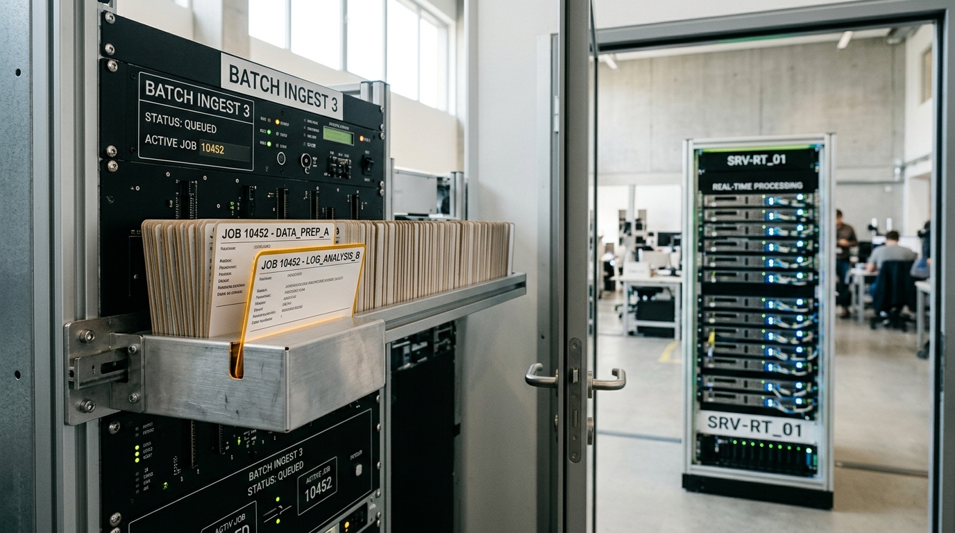
Figure 5. Batch processing sells the provider a right to delay in exchange for a lower price; real-time serving pays a premium for the promise that nothing waits. — Image prompt and art direction by Brecht Corbeel; generation pending.

The comparison that does not survive this axis is “batch is cheaper than real-time,” stated as a general claim about cost per unit of computation. It is not: the discount is a price for a scheduling property — the freedom to delay — not for less arithmetic. A workload that must answer a user in under a second has no batch option regardless of price, and a workload that can tolerate a lengthy turnaround is choosing to sell that tolerance back to the provider at a fixed, published rate rather than proving that asynchronous computation is intrinsically cheaper to perform.

Why these axes do not collapse into one ranking

Five axes — hosting model, architecture, capacity commitment, precision and processing mode — combine multiplicatively rather than in a line, and the evidence gathered for this article covers each axis on its own terms without covering the combinations. A self-hosted fleet running a quantized mixture-of-experts model on reserved capacity for batch workloads is a real, buildable configuration; nothing published by any vendor or paper cited here prices that specific configuration against, say, API access to a dense model at standard synchronous pricing, because no single source spans both. Comparing the two responsibly means measuring a workload against each axis separately — its own utilization rate against the reserved-versus-on-demand break-even above, its own task’s tolerance for a 3-to-4-bit model against its own evaluation suite, its own request pattern’s tolerance for delay against the batch discount on its rate card — rather than importing a ranking built for someone else’s traffic.

This is also why total cost of ownership resists a single number more than any individual line item does. A self-hosted or colocated deployment carries capital cost, the electricity draw the IEA documents growing at roughly 12 percent a year industry-wide [17], facility overhead, and the engineering team that builds and operates the serving stack, none of which appears on any competing API rate card. An API or managed-platform price has all of that folded in already, priced by a vendor whose own utilization, hardware generation and negotiated hardware costs are not disclosed. Neither figure is wrong. They are answers to different questions, and the discipline this comparison calls for is not picking a winner across them but being precise about which question a given number actually answers before using it to decide anything.

What to take away

None of the five axes compared here reduces to “which is cheaper” as a standalone question, and every attempt in this piece to state one plainly has run into a workload-specific variable the published sources cannot supply: a utilization rate for hosting, a task’s tolerance for precision loss, a request pattern’s tolerance for delay. The one place a clean, general model was available — the break-even utilization at which reserved capacity beats paying on demand — turned out to require exactly one number only the buyer holds. That is not a failure of the comparison; it is what an honest comparison across incomparable conditions looks like; the alternative, forcing five separate markets into a single ranked list, would be a confident-sounding number built on data that does not support it. The more durable habit is the one this article has tried to model throughout: name the axis, cite what is actually published about it, and stop exactly where the workload — not the vendor — has to supply the missing term.

Sources

1. Amazon Web Services. EC2 On-Demand Instance Pricing. AWS Documentation (2026).
2. Amazon Web Services. Amazon EC2 Spot Instances Pricing. AWS Documentation (2026).
3. Amazon Web Services. Spot Instance Advisor. AWS Documentation (2026).
4. Amazon Web Services. Compute Savings Plans Pricing. AWS Documentation (2026).
5. Amazon Web Services. Amazon EC2 P5 Instances. AWS Documentation (2026).
6. CoreWeave. GPU Cloud Pricing. CoreWeave (2026).
7. Microsoft. Provisioned Throughput for Foundry Models. Microsoft Learn (2026).
8. Together AI. Pricing. Together AI (2026).
9. Anthropic. Pricing. Claude Platform Documentation (2026).
10. OpenAI. API Pricing. OpenAI Platform Documentation (2026).
11. DeepSeek-AI. DeepSeek-V3 Technical Report. arXiv (2024). DOI: 10.48550/arXiv.2412.19437.
12. Albert Q. Jiang et al.. Mixtral of Experts. arXiv (2024). DOI: 10.48550/arXiv.2401.04088.
13. William Fedus, Barret Zoph, and Noam Shazeer. Switch Transformers: Scaling to Trillion Parameter Models with Simple and Efficient Sparsity. arXiv (2021). DOI: 10.48550/arXiv.2101.03961.
14. Elias Frantar, Saleh Ashkboos, Torsten Hoefler, and Dan Alistarh. GPTQ: Accurate Post-Training Quantization for Generative Pre-trained Transformers. arXiv (2022). DOI: 10.48550/arXiv.2210.17323.
15. Ji Lin et al.. AWQ: Activation-Aware Weight Quantization for LLM Compression and Acceleration. arXiv (2023). DOI: 10.48550/arXiv.2306.00978.
16. NVIDIA. NVIDIA Hopper Architecture. NVIDIA (2026).
17. International Energy Agency. Energy and AI: Executive Summary. International Energy Agency (2025).
18. Reiner Pope et al.. Efficiently Scaling Transformer Inference. Proceedings of Machine Learning and Systems (2023). DOI: 10.48550/arXiv.2211.05102.
19. Woosuk Kwon et al.. Efficient Memory Management for Large Language Model Serving with PagedAttention. ACM Symposium on Operating Systems Principles (2023). DOI: 10.48550/arXiv.2309.06180.

Originally published at https://absolutedigitalpublishers.com/articles/comparing-the-main-approaches-to-ai-inference-economics.